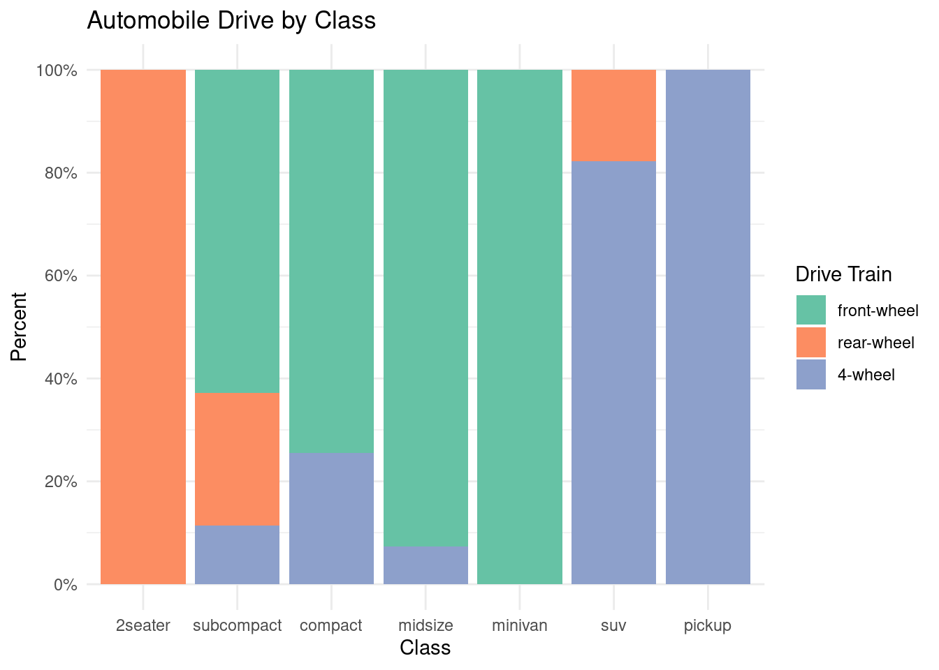
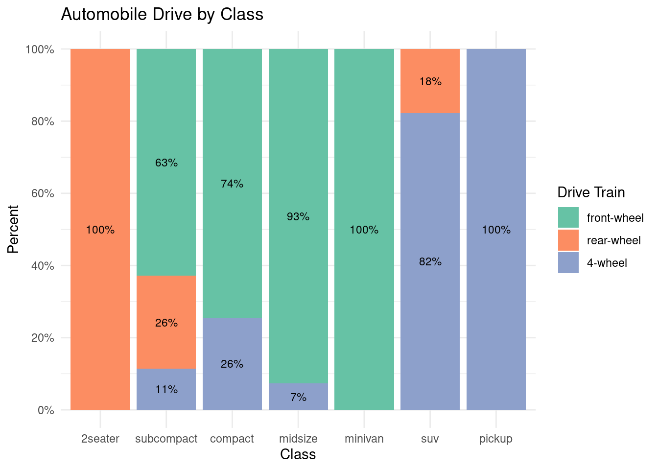
Improving the color and labeling
library(ggplot2)

# bar plot, with each bar representing 100%,
# reordered bars, and better labels and colors
library(scales)
ggplot(mpg,
  aes(x = factor(class,
  levels = c("2seater", "subcompact",
  "compact", "midsize", "minivan", "suv", "pickup")), fill = factor(drv,
levels = c("f", "r", "4"),
labels = c("front-wheel", "rear-wheel",
          "4-wheel")))) +
  geom_bar(position = "fill") +
  scale_y_continuous(breaks = seq(0, 1, .2),
                     label = percent) +
  scale_fill_brewer(palette = "Set2") +
  labs(y = "Percent",
       fill = "Drive Train",
       x = "Class",
       title = "Automobile Drive by Class") +
  theme_minimal()

# create a summary dataset
library(dplyr)
plotdata <- mpg %>%
  group_by(class, drv) %>%
  summarize(n = n()) %>%
  mutate(pct = n/sum(n),
         lbl = scales::percent(pct))
## `summarise()` has grouped output by 'class'. You can override using the
## `.groups` argument.
## # A tibble: 12 × 5
## # Groups:   class [7]
##    class      drv       n    pct lbl
##    <chr>      <chr> <int>  <dbl> <chr>
##  1 2seater    r         5 1      100%
##  2 compact    4        12 0.255  26%
##  3 compact    f        35 0.745  74%
##  4 midsize    4         3 0.0732 7%
##  5 midsize    f        38 0.927  93%
##  6 minivan    f        11 1      100%
##  7 pickup     4        33 1      100%
##  8 subcompact 4         4 0.114  11%
##  9 subcompact f        22 0.629  63%
## 10 subcompact r         9 0.257  26%
## 11 suv        4        51 0.823  82%
## 12 suv        r        11 0.177  18%
ggplot(plotdata,
  aes(x = factor(class,
  levels = c("2seater", "subcompact",
  "compact", "midsize", "minivan", "suv", "pickup")),y = pct,
  fill = factor(drv, levels = c("f", "r", "4"),
  labels = c("front-wheel","rear-wheel",
  "4-wheel")))) +
  geom_bar(stat = "identity",
           position = "fill") +
  scale_y_continuous(breaks = seq(0, 1, .2),
                     label = percent) +
  geom_text(aes(label = lbl),
            size = 3,
            position = position_stack(vjust = 0.5)) +
  scale_fill_brewer(palette = "Set2") +
  labs(y = "Percent",
       fill = "Drive Train",
       x = "Class",
       title = "Automobile Drive by Class") +
  theme_minimal()


