8.7 Another linear regression example

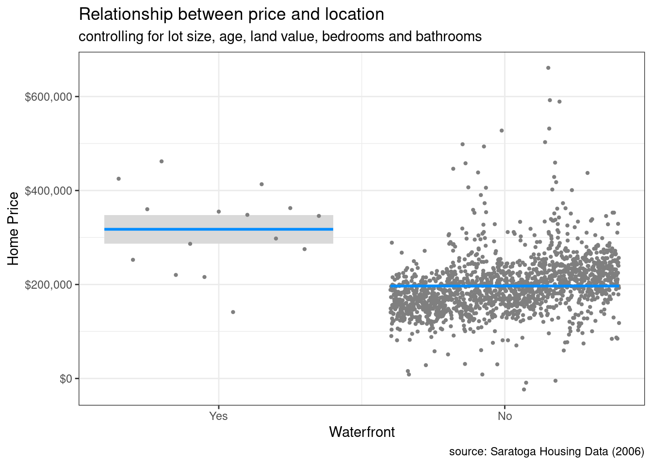
• Continuing the example, the price difference between waterfront and non-waterfront homes is plotted, controlling for the other seven variables.

• Since a ggplot2 graph is produced, other ggplot2 functions can be added to customize the graph.

# conditional plot of price vs. waterfront location
visreg(houses_lm, "waterfront", gg = TRUE) +
  scale_y_continuous(label = scales::dollar) +
  labs(title = "Relationship between price and location",
       subtitle = "controlling for lot size, age, land value, bedrooms and bathrooms",
       caption = "source: Saratoga Housing Data (2006)",
       y = "Home Price",
       x = "Waterfront")

• We see that there are far fewer homes on the water, and they tend to be more expensive (even controlling for size, age, and land value).