11.3 Utilizing two predictors

What we know about afternoon temperatures in Australia:

• positively associated with morning temperatures
• tend to be lower in Wollongong than in Uluru

Now extend the model to:

two-predictor model of 3 p.m. temperature using both temp9am and location

ggplot(weather_WU, aes(y = temp3pm, 
                       x = temp9am, 
                       color = location)) + 
  geom_point() + 
  geom_smooth(method = "lm", se = FALSE)

## `geom_smooth()` using formula = 'y ~ x'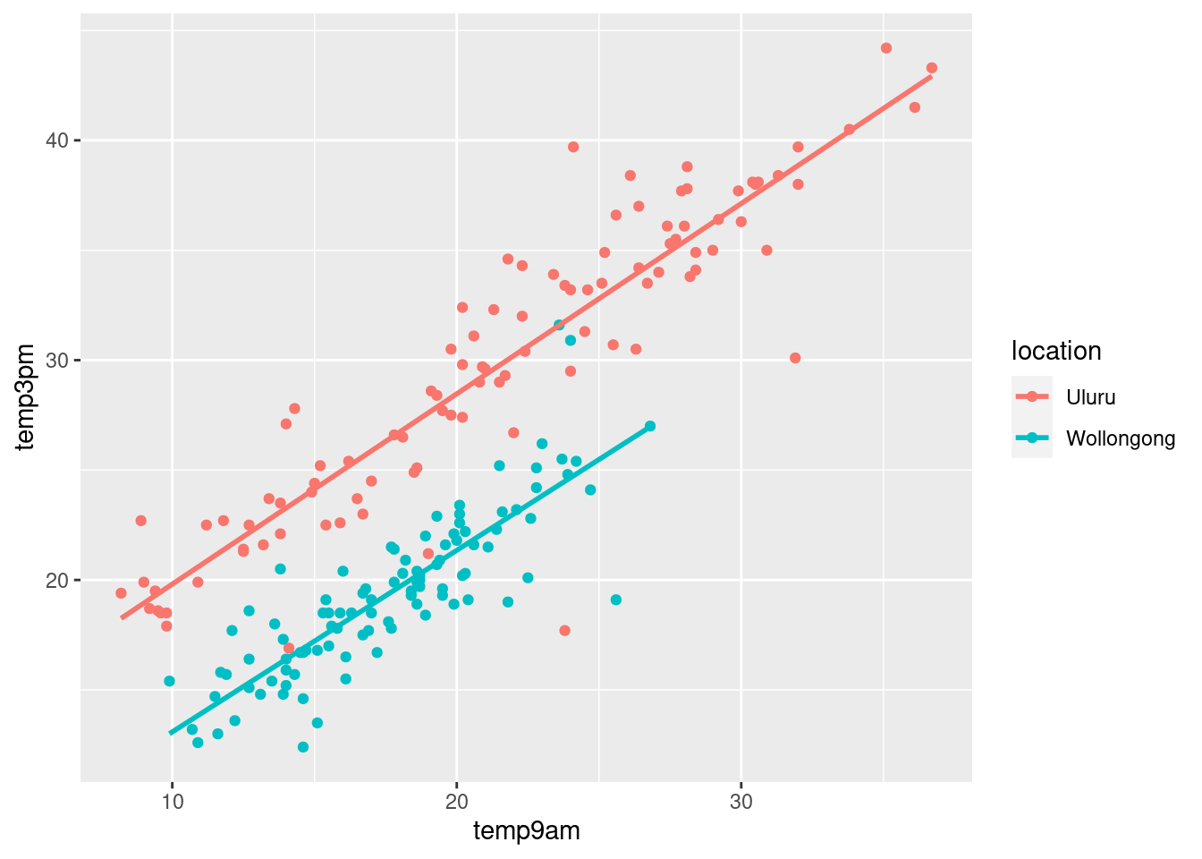

weather_model_3_prior <- stan_glm(
  temp3pm ~ temp9am + location,
  data = weather_WU, 
  family = gaussian, 
  prior_intercept = normal(25, 5),
  prior = normal(0, 2.5, autoscale = TRUE), 
  prior_aux = exponential(1, autoscale = TRUE),
  chains = 4, 
  iter = 5000*2, 
  seed = 84735,
  prior_PD = TRUE)

11.3.1 Simulate 100 datasets from the prior models

set.seed(84735)
weather_WU %>%
  add_predicted_draws(weather_model_3_prior, n = 100) %>%
  ggplot(aes(x = .prediction, group = .draw)) +
    geom_density() + 
    xlab("temp3pm")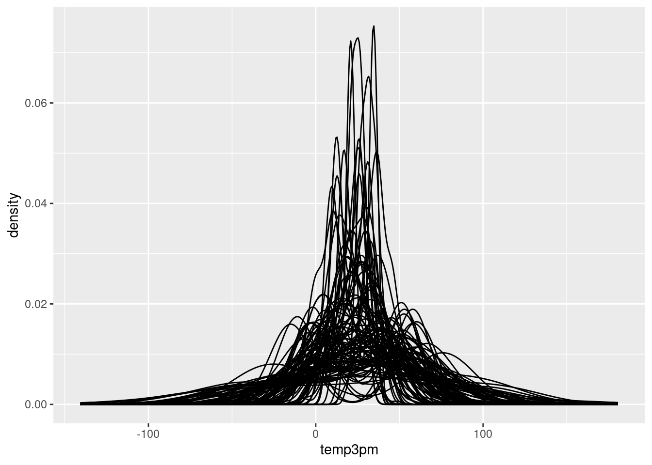

weather_WU %>%
  add_fitted_draws(weather_model_3_prior, n = 100) %>%
  ggplot(aes(x = temp9am, 
             y = temp3pm, 
             color = location)) +
    geom_line(aes(y = .value, 
                  group = paste(location, .draw)))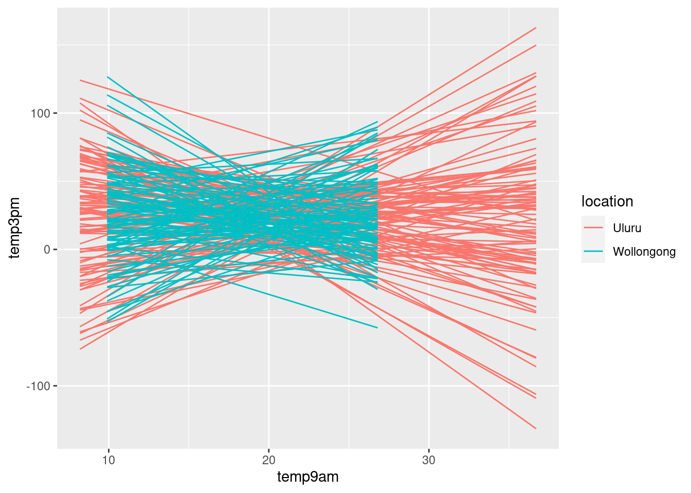

Combine prior assumption with simulations, specifying

prior_PD = FALSE

weather_model_3 <- update(weather_model_3_prior,
                          prior_PD = FALSE)

Across all 100 scenarios, 3 p.m. temperature is positively associated with 9 a.m. temperature and tends to be higher in Uluru than in Wollongong.

head(as.data.frame(weather_model_3), 6)

##   (Intercept)   temp9am locationWollongong    sigma
## 1    13.04657 0.8016891          -7.663020 2.392109
## 2    12.73136 0.8174191          -7.838690 2.444850
## 3    11.81295 0.8615380          -7.647937 2.413606
## 4    12.37991 0.8041587          -6.845878 2.552823
## 5    12.22305 0.8391698          -7.419569 2.498952
## 6    10.94792 0.8539339          -6.821811 2.272895

weather_WU %>%
  add_fitted_draws(weather_model_3, n = 100) %>%
  ggplot(aes(x = temp9am, y = temp3pm, color = location)) +
    geom_line(aes(y = .value, group = paste(location, .draw)), alpha = .1) +
    geom_point(data = weather_WU, size = 0.1)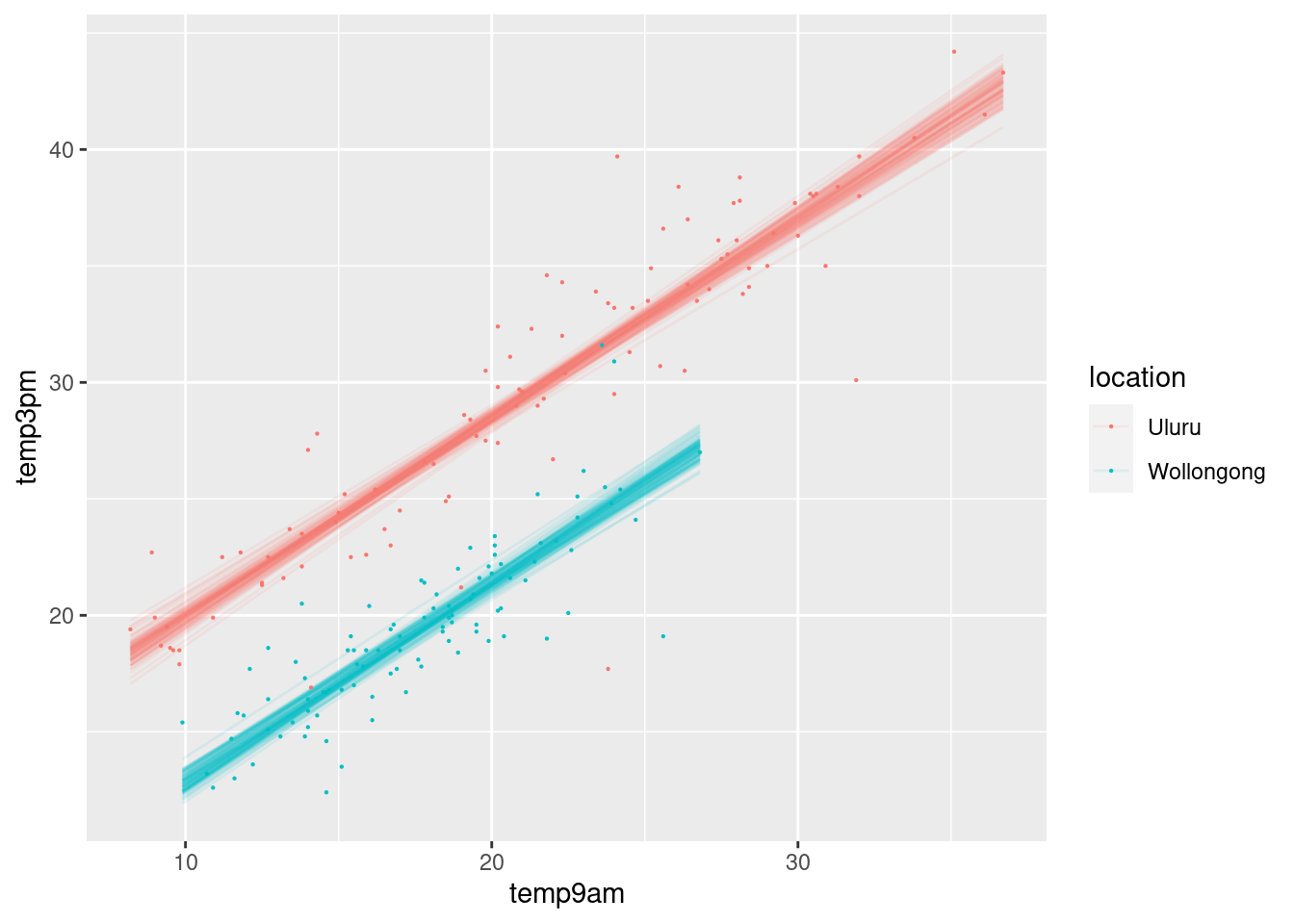

# Posterior summaries
posterior_interval(weather_model_3, prob = 0.80, 
                   pars = c("temp9am", "locationWollongong"))

##                           10%        90%
## temp9am             0.8196281  0.8945346
## locationWollongong -7.5067716 -6.5999057

11.3.2 Predict 3 p.m. temperature on specific days

# Simulate a set of predictions
set.seed(84735)
temp3pm_prediction <- posterior_predict(
  weather_model_3,
  newdata = data.frame(temp9am = c(10, 10), 
                       location = c("Uluru", "Wollongong")))

# Plot the posterior predictive models
mcmc_areas(temp3pm_prediction) +
  ggplot2::scale_y_discrete(labels = c("Uluru", "Wollongong")) + 
  xlab("temp3pm")

## Scale for y is already present.
## Adding another scale for y, which will replace the existing scale.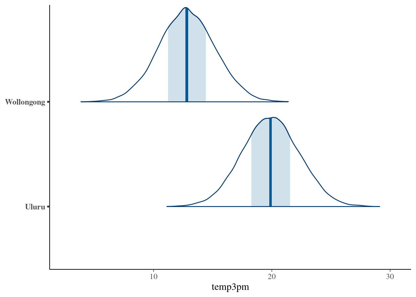

## Optional: Utilizing interaction terms

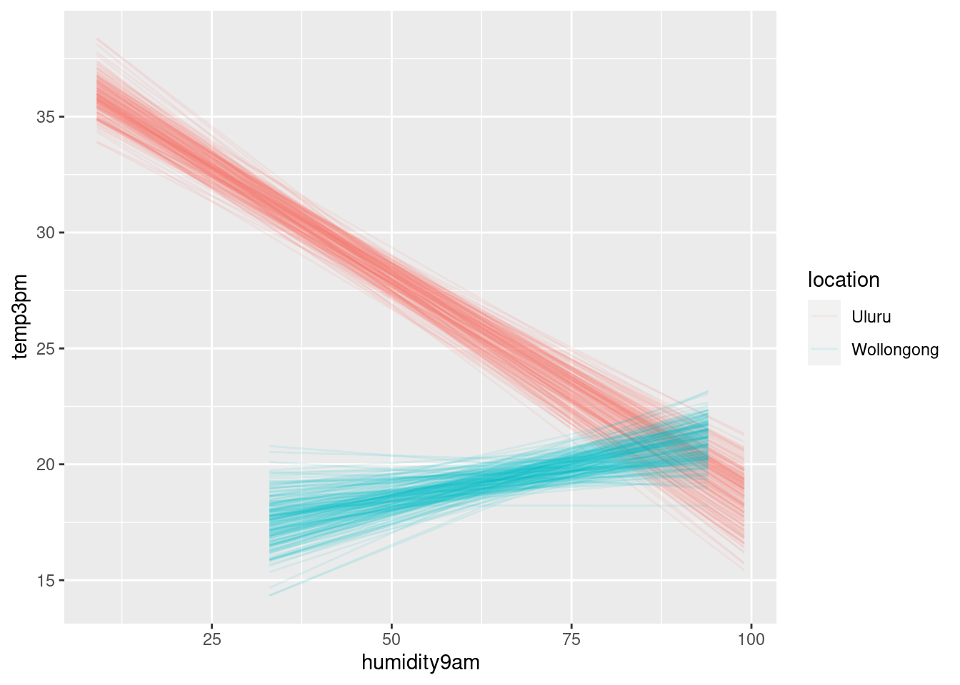
Predictors interaction of 3 p.m. temperature (\(Y\)) with location (\(X_2\)) and 9 a.m. humidity (\(X_3\)).

ggplot(weather_WU, aes(y = temp3pm, 
                       x = humidity9am, 
                       color = location)) +
  geom_point(size = 0.5) + 
  geom_smooth(method = "lm", se = FALSE)

## `geom_smooth()` using formula = 'y ~ x'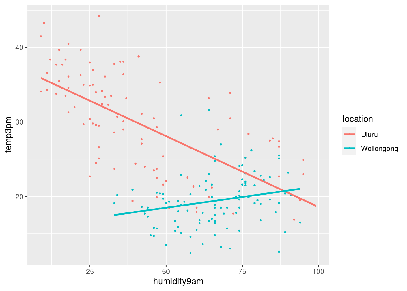

interaction_model <- stan_glm(
  temp3pm ~ location + humidity9am + location:humidity9am, 
  data = weather_WU, family = gaussian,
  prior_intercept = normal(25, 5),
  prior = normal(0, 2.5, autoscale = TRUE), 
  prior_aux = exponential(1, autoscale = TRUE),
  chains = 4, iter = 5000*2, seed = 84735)

# Posterior summary statistics
tidy(interaction_model, effects = c("fixed", "aux"))

## # A tibble: 6 × 3
##   term                           estimate std.error
##   <chr>                             <dbl>     <dbl>
## 1 (Intercept)                      37.6      0.909 
## 2 locationWollongong              -21.8      2.31  
## 3 humidity9am                      -0.190    0.0193
## 4 locationWollongong:humidity9am    0.246    0.0372
## 5 sigma                             4.47     0.229 
## 6 mean_PPD                         24.6      0.453

Simulations:

weather_WU %>%
  add_fitted_draws(interaction_model, n = 200) %>%
  ggplot(aes(x = humidity9am, 
             y = temp3pm, 
             color = location)) +
    geom_line(aes(y = .value, group = paste(location, .draw)), alpha = 0.1)

## Warning: `fitted_draws` and `add_fitted_draws` are deprecated as their names were confusing.
## - Use [add_]epred_draws() to get the expectation of the posterior predictive.
## - Use [add_]linpred_draws() to get the distribution of the linear predictor.
## - For example, you used [add_]fitted_draws(..., scale = "response"), which
##   means you most likely want [add_]epred_draws(...).
## NOTE: When updating to the new functions, note that the `model` parameter is now
##   named `object` and the `n` parameter is now named `ndraws`.