6.4 Beta Binomial Example

\[\begin{array}{rcl} \pi & \sim & \text{Beta}(2,2) \\ Y|\pi & \sim & \text{Bin}(10,\pi)\\ \end{array}\]

\[\text{E}(\pi) = \frac{\alpha}{\alpha + \beta} = \frac{2}{2 + 2} = 0.5\]

• We bbserve \(Y=9\) successes (out of 10)

# Step 1: Define grid
grid_data <- data.frame(pi_grid = seq(from = 0, to = 1, length = 100))

# Step 2: Evaluate numerator
grid_data <- grid_data %>% 
  mutate(prior = dbeta(pi_grid, 2, 2),
         likelihood = dbinom(9, 10, pi_grid)) %>%
  mutate( unnormalized = prior*likelihood)

# Step 3: Normalize! 
grid_data <- grid_data %>% 
   mutate(posterior = unnormalized/sum(unnormalized))

ggplot(grid_data, aes(x = pi_grid, y = posterior)) + 
  geom_point() + 
  geom_segment(aes(x = pi_grid, xend = pi_grid, y = 0, yend = posterior))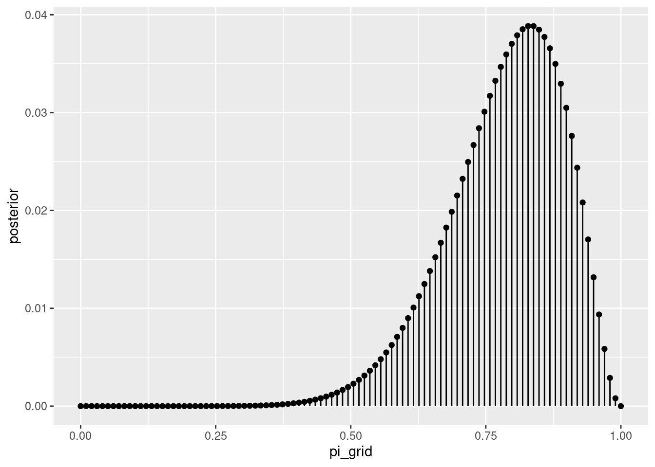

• Sample from this posterior (Step 4)

set.seed(84735)  #BAYES
post_sample <- sample_n(grid_data, size = 10000, weight = posterior, replace = TRUE)
ggplot(post_sample, aes(x = pi_grid)) + 
  geom_histogram(aes(y = after_stat(density)), color = "white", binwidth = 0.05) + 
  stat_function(fun = dbeta, args = list(11, 3)) + 
  lims(x = c(0, 1))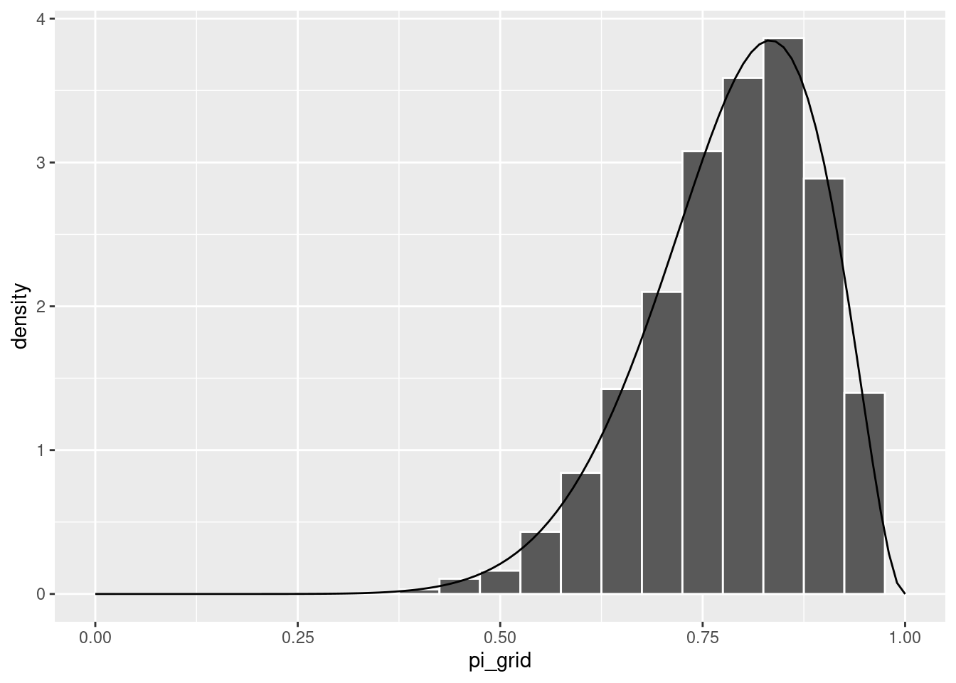

• We can compute any summary statistics from the samples (or from the grid posterior itself!)

\[\text{E}(\pi) = \frac{\alpha}{\alpha + \beta} = \frac{11}{11 + 3} \approx 0.7857\]