16.5 Posterior prediction

What will be the popularity of new song of artist j (two cases: artist in the data / unknown artist)?

posterior_predict() exist but first we do it by “hand”!

16.5.1 First case: Frank Ocean (j=39)

\[Y^{i}_{new,j} | \mu_j, \sigma_y \sim N(\mu_j^{i}, (\sigma^{(i)}_y)^2)\]

We have plenty of \(\mu^{i}_j\) and \(\sigma^{(i)}_y\) with two sources of variability :

Not all song of Ocean are eqully popular (within-group sampling variability)
we do not know the exact mean and variability of Ocean song (posterior variability)

# Simulate Ocean's posterior predictive model
set.seed(84735)
ocean_chains <- spotify_hierarchical_df |>
  rename(b = `b[(Intercept) artist:Frank_Ocean]`) |> 
  select(`(Intercept)`, b, sigma) |> 
  mutate(mu_ocean = `(Intercept)` + b,
         y_ocean = rnorm(20000, mean = mu_ocean, sd = sigma)) # stuff that I always forget

# Check it out
head(ocean_chains, 3)

##   (Intercept)        b    sigma mu_ocean  y_ocean
## 1    49.93503 18.01483 14.51838 67.94986 77.63700
## 2    49.20877 19.15738 13.47368 68.36615 66.69757
## 3    51.66700 19.05753 14.27727 70.72453 81.87319

Then you summarize it:

ocean_chains |> 
  mean_qi(y_ocean, .width = 0.80)

## # A tibble: 1 × 6
##   y_ocean .lower .upper .width .point .interval
##     <dbl>  <dbl>  <dbl>  <dbl> <chr>  <chr>    
## 1    69.4   51.4   87.6    0.8 mean   qi

# to put into context 
# the range of a new song is wider tham the average of ocean
artist_summary_scaled |>
  filter(artist == "artist:Frank_Ocean")

## # A tibble: 1 × 7
##   artist              mu_j .lower .upper .width .point .interval
##   <fct>              <dbl>  <dbl>  <dbl>  <dbl> <chr>  <chr>    
## 1 artist:Frank_Ocean  69.4   66.6   72.2    0.8 mean   qi

16.5.2 Posterior prediction for an observed group

We do not have \(\mu_j\) but we know new artist is an artist! And we now the range of mean popularity level among artist \(N(\mu, \sigma_u)\) and we have 44 artists.

step 1: simulate \(\mu_{new_artist}\) bt drawing into layer 2 of MCMC
step 2: simulate song popularity with Layer 1 and \(\mu_{new_artist}\)

We are adding a new source of variability (not all artist are equally popular : between group)

set.seed(84735)
mohsen_chains <- spotify_hierarchical_df |>
  mutate(sigma_mu = sqrt(`Sigma[artist:(Intercept),(Intercept)]`),
         mu_mohsen = rnorm(20000, `(Intercept)`, sigma_mu), # new stuff
         y_mohsen = rnorm(20000, mu_mohsen, sigma))

# Posterior predictive summaries
mohsen_chains |> 
  mean_qi(y_mohsen, .width = 0.80)

## # A tibble: 1 × 6
##   y_mohsen .lower .upper .width .point .interval
##      <dbl>  <dbl>  <dbl>  <dbl> <chr>  <chr>    
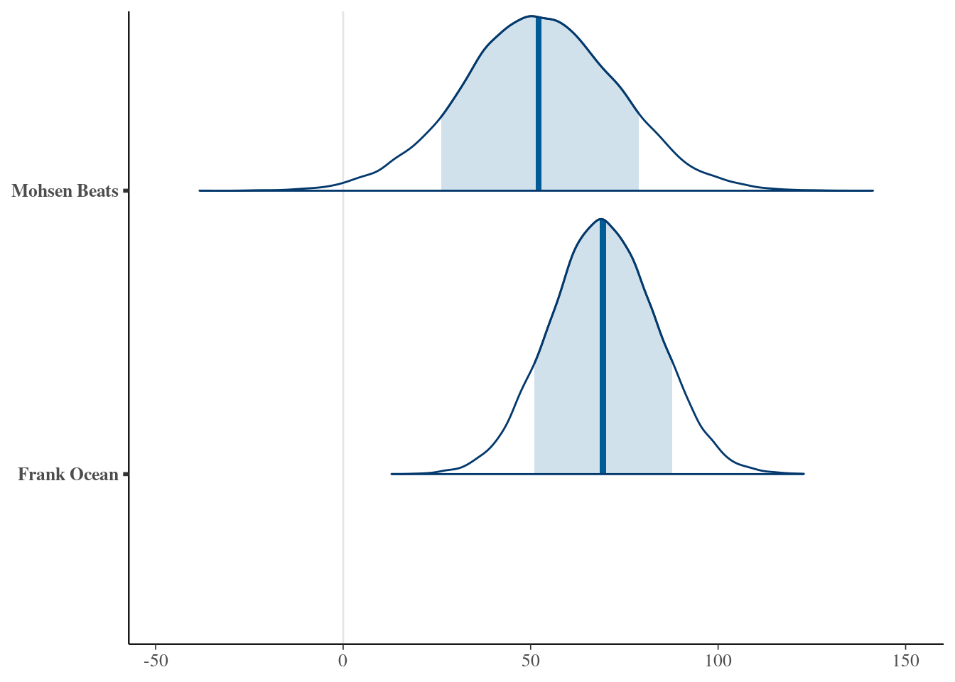
## 1     52.3   25.9   78.8    0.8 mean   qi

16.5.3 posterior_predict()

set.seed(84735)
prediction_shortcut <- posterior_predict(
  spotify_hierarchical,
  newdata = data.frame(artist = c("Frank Ocean", "Mohsen Beats")))

# Posterior predictive model plots
mcmc_areas(prediction_shortcut, prob = 0.8) +
  ggplot2::scale_y_discrete(labels = c("Frank Ocean", "Mohsen Beats"))

## Scale for y is already present.
## Adding another scale for y, which will replace the existing scale.