13.3 Prediction & classification

weather%>%pull(humidity9am)%>%range()

## [1] 13 99

Posterior predictions of binary outcome:

set.seed(84735)
binary_prediction <- posterior_predict(
  rain_model_1, 
  newdata = data.frame(humidity9am = 99))

set.seed(84735)
rain_model_1_df <- as.data.frame(rain_model_1) %>% 
  mutate(log_odds = `(Intercept)` + humidity9am*99,
         odds = exp(log_odds),
         prob = odds / (1 + odds),
         Y = rbinom(20000, size = 1, prob = prob))

rain_model_1_df %>% head

##   (Intercept) humidity9am    log_odds      odds      prob Y
## 1   -4.244453  0.04454776  0.16577499 1.1803075 0.5413491 0
## 2   -4.207118  0.04209875 -0.03934156 0.9614223 0.4901659 1
## 3   -3.899987  0.03877941 -0.06082497 0.9409879 0.4847984 0
## 4   -3.942503  0.03948000 -0.03398243 0.9665885 0.4915052 1
## 5   -4.743743  0.05139157  0.34402150 1.4106090 0.5851671 0
## 6   -4.405777  0.04565130  0.11370120 1.1204173 0.5283947 1

weather%>%
  group_by(raintomorrow)%>%
  reframe(avg=mean(humidity9am))%>%
  mutate(prop=avg/sum(avg))

## # A tibble: 2 × 3
##   raintomorrow   avg  prop
##   <fct>        <dbl> <dbl>
## 1 No            58.4 0.449
## 2 Yes           71.6 0.551

mcmc_hist(binary_prediction) + 
  labs(x = "Y")

## `stat_bin()` using `bins = 30`. Pick better value with `binwidth`.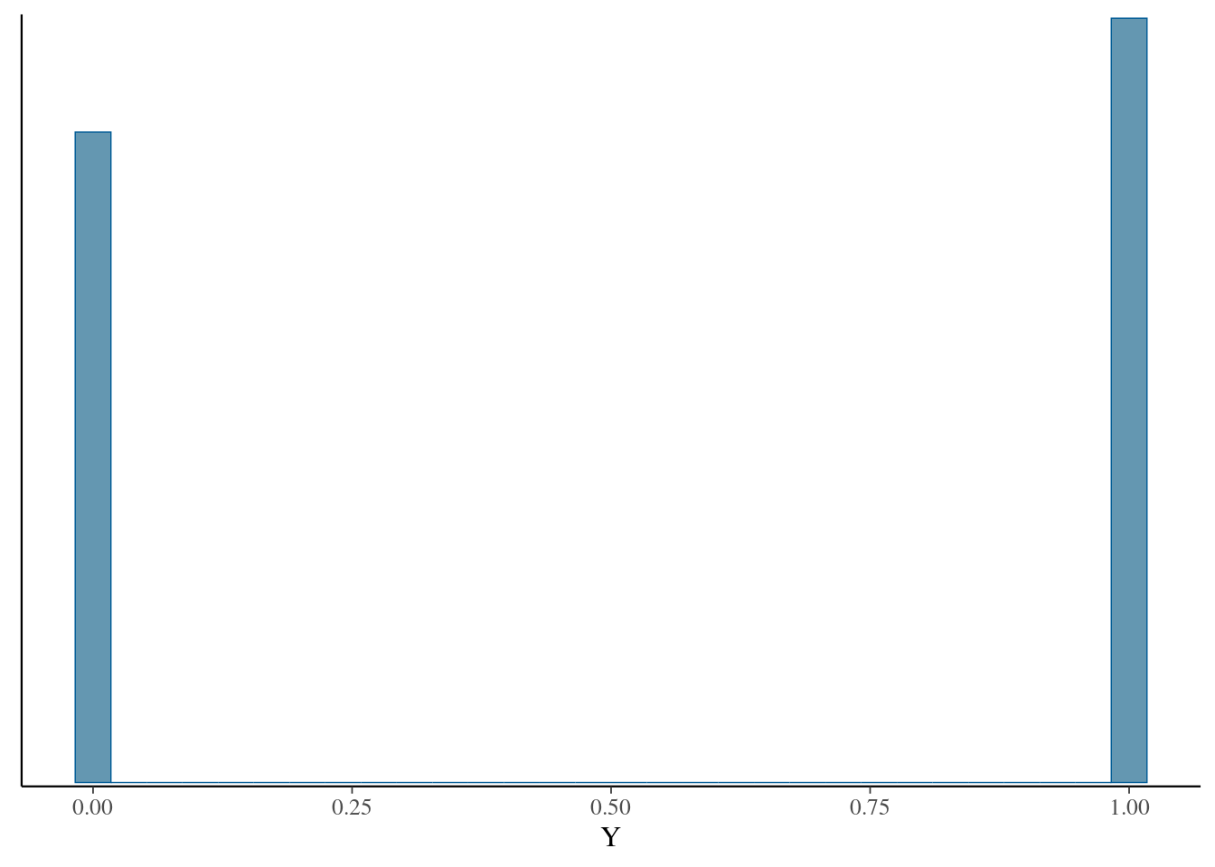

ggplot(rain_model_1_df, aes(x = Y)) + 
  stat_count()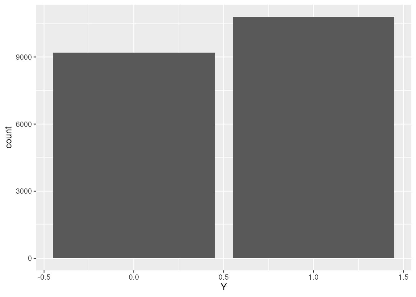

# Summarize the posterior predictions of Y
table(binary_prediction)

## binary_prediction
##     0     1 
##  9196 10804

colMeans(binary_prediction)

##      1 
## 0.5402