18.2 Hierarchical logistic regression
# Load packages
library(bayesrules)
library(tidyverse)
library(bayesplot)
library(rstanarm)
library(tidybayes)
library(broom.mixed)
library(janitor)

climbers <- climbers_sub %>%
  select(expedition_id, member_id, success, year, season,
         age, expedition_role, oxygen_used)
Data are from The Himalayan Database, Himalayan Climbing Expeditions data shared through the #tidytuesday project R for Data Science 2020b, made of 2076 climbers, dating back to 1978.
# Import, rename, & clean data
data(climbers_sub)
climbers <- climbers_sub %>%
  select(expedition_id, member_id, success, year, season,
         age, expedition_role, oxygen_used)
nrow(climbers)
## [1] 2076climbers%>%head# A tibble: 6 × 8
expedition_id member_id success year season age expedition_role oxygen_used
<chr> <fct> <lgl> <dbl> <fct> <dbl> <fct> <lgl>
1 AMAD81101 AMAD8110… TRUE 1981 Spring 28 Climber FALSE
2 AMAD81101 AMAD8110… TRUE 1981 Spring 27 Exp Doctor FALSE
3 AMAD81101 AMAD8110… TRUE 1981 Spring 35 Deputy Leader FALSE
4 AMAD81101 AMAD8110… TRUE 1981 Spring 37 Climber FALSE
5 AMAD81101 AMAD8110… TRUE 1981 Spring 43 Climber FALSE
6 AMAD81101 AMAD8110… FALSE 1981 Spring 38 Climber FALSE To generate a frequency table we use the tabyl() function:
?janitor::tabylclimbers %>%
janitor::tabyl(success) success n percent
FALSE 1269 0.6112717
TRUE 807 0.3887283# Size per expedition
climbers_per_expedition <- climbers %>% count(expedition_id)
# Number of expeditions
nrow(climbers_per_expedition)## [1] 200The individual climber outcomes are independent.
climbers_per_expedition %>%
  head(3)
## # A tibble: 3 × 2
## expedition_id n
## <chr> <int>
## 1 AMAD03107 5
## 2 AMAD03327 6
## 3 AMAD05338 12More than 75 of our 200 expeditions had a 0% success rate. In contrast, nearly 20 expeditions had a 100% success rate.
There’s quite a bit of variability in expedition success rates.
# Calculate the success rate for each exhibition
expedition_success <- climbers %>%
  group_by(expedition_id) %>%
  summarize(success_rate = mean(success))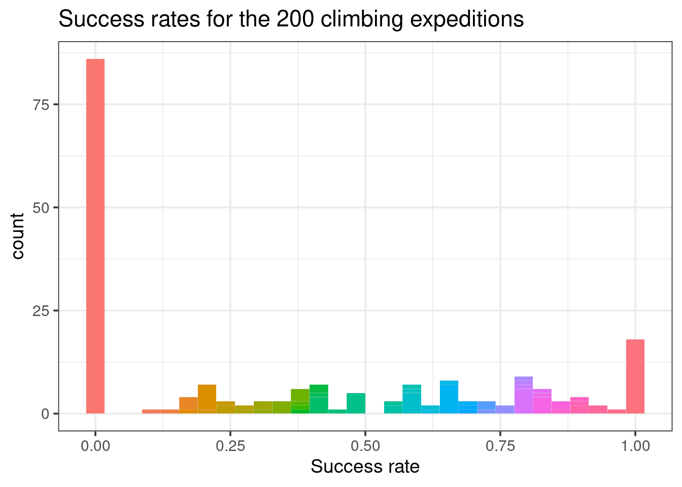
Figure 18.2: Histogram of the success rates for the 200 climbing expeditions
18.2.1 Model building & simulation
We use the Bernoulli model for binary response variable: expedtion success
\[Y_{ij}=\left\{\begin{matrix} 0 & \text{yes} \\ 1 & \text{no} \end{matrix}\right.\]
\[X_{ij1}= \text{age of climber j in expedition j}\] \[X_{ij2}= \text{climber i received oxygen in expedition j}\]
Bayesian model
\[Y_{ij}|\pi_{ij}\sim Bern(\pi_{ij})\] Complete pooling expands this simple model into a logistic regression model
\[Y_{ij}|\beta_0,\beta_1,\beta_2\overset{ind}\sim Bern(\pi_{ij})\]
with
- \(\beta_0\) the typical baseline success rate across all expeditions
- \(\beta_1\) the global relationship between success and age when controlling for oxygen use
- \(\beta_2\) the global relationship between success and oxygen use when **controlling for age
\[log(\frac{\pi_{ij}}{1-\pi_{ij}})=\beta_0+\beta_1X_{ij1}+\beta_2X_{ij2}\] We need to take account for the grouping structure of our data.
# Calculate the success rate by age and oxygen use
data_by_age_oxygen <- climbers %>%
  group_by(age, oxygen_used) %>%
  summarize(success_rate = mean(success),.groups="drop")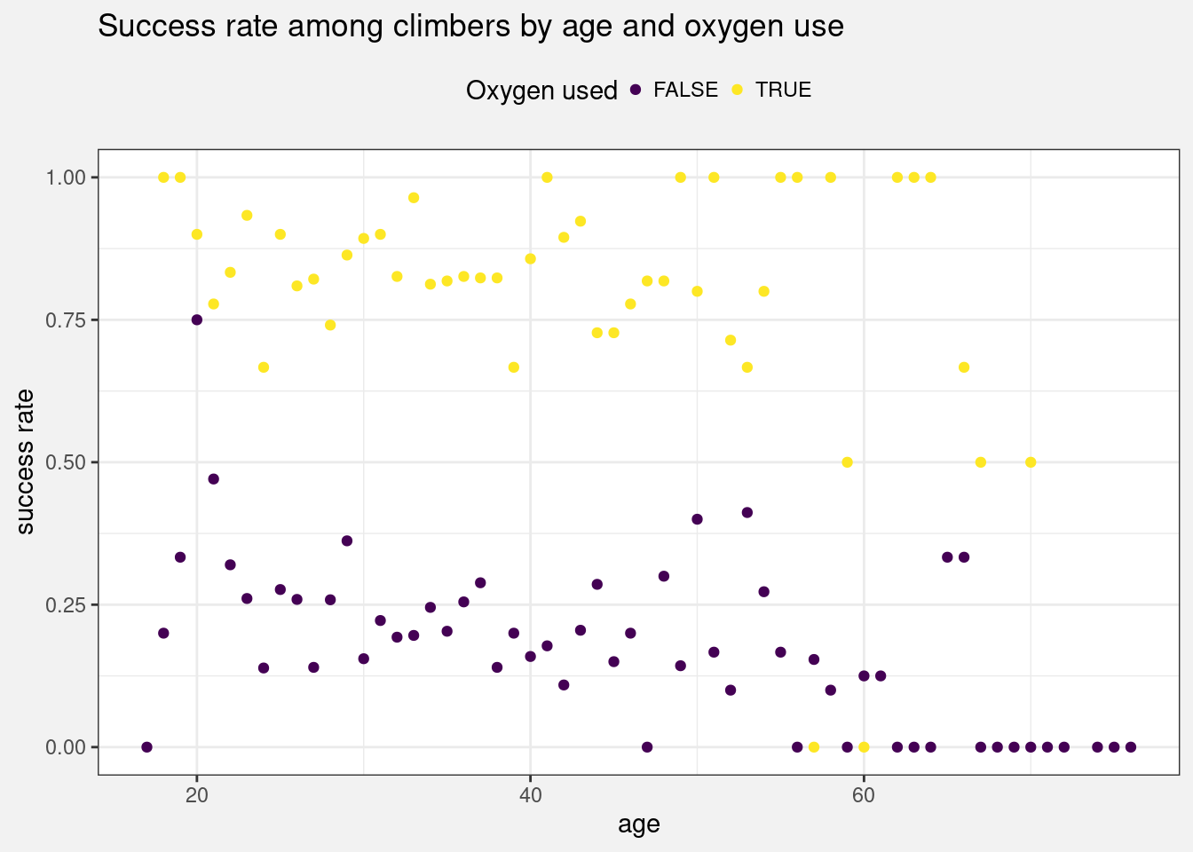
Figure 18.3: Scatterplot of the success rate among climbers by age and oxygen use
We substitute \(\beta_0\) with the centered intercept \(\beta_{0c}\).
\[\beta_{0c}\sim N(m_0,s_0^2)\]
\(m_0=0\) and \(s_0^2=2.5^2\), \(s_1^2=0.24^2\), \(s_2^2=5.51^2\)
\[\beta_{0j}|\beta_0,\sigma_0\overset{ind}\sim N(\beta_0,s_0^2)\]
and,
\[\sigma_0\sim Exp(1)\]
Reframe the random intercepts logistic regression model as a tweaks to the global intercept:
\[log(\frac{\pi_{ij}}{1-\pi_{ij}})=(\beta_0+b_{0j})+\beta_1X_{ij1}+\beta_2X_{ij2}\]
- \(b_{0j}\) depends on the variability
\[b_{0j}|\sigma_0\overset{ind}\sim N(0,\sigma_0^2)\]
- \(\sigma_0\) captures the between-group variability in success rates from expedition to expedition
Set the model formula to hierarchical grouping structure:
success ~ age + oxygen_used + (1 | expedition_id)climb_model <- stan_glmer(
success ~ age + oxygen_used + (1 | expedition_id),
data = climbers, family = binomial,
prior_intercept = normal(0, 2.5, autoscale = TRUE),
prior = normal(0, 2.5, autoscale = TRUE),
prior_covariance = decov(reg = 1, conc = 1, shape = 1, scale = 1),
chains = 4, iter = 5000*2, seed = 84735
)Confirm prior specifications
prior_summary(climb_model)MCMC diagnostics
mcmc_trace(climb_model, size = 0.1)
mcmc_dens_overlay(climb_model)
mcmc_acf(climb_model)
neff_ratio(climb_model)
rhat(climb_model)
Define success rate function
success_rate <- function(x){mean(x == 1)}Posterior predictive check
pp_check(climb_model, nreps = 100,
         plotfun = "stat", stat = "success_rate") +
  xlab("success rate")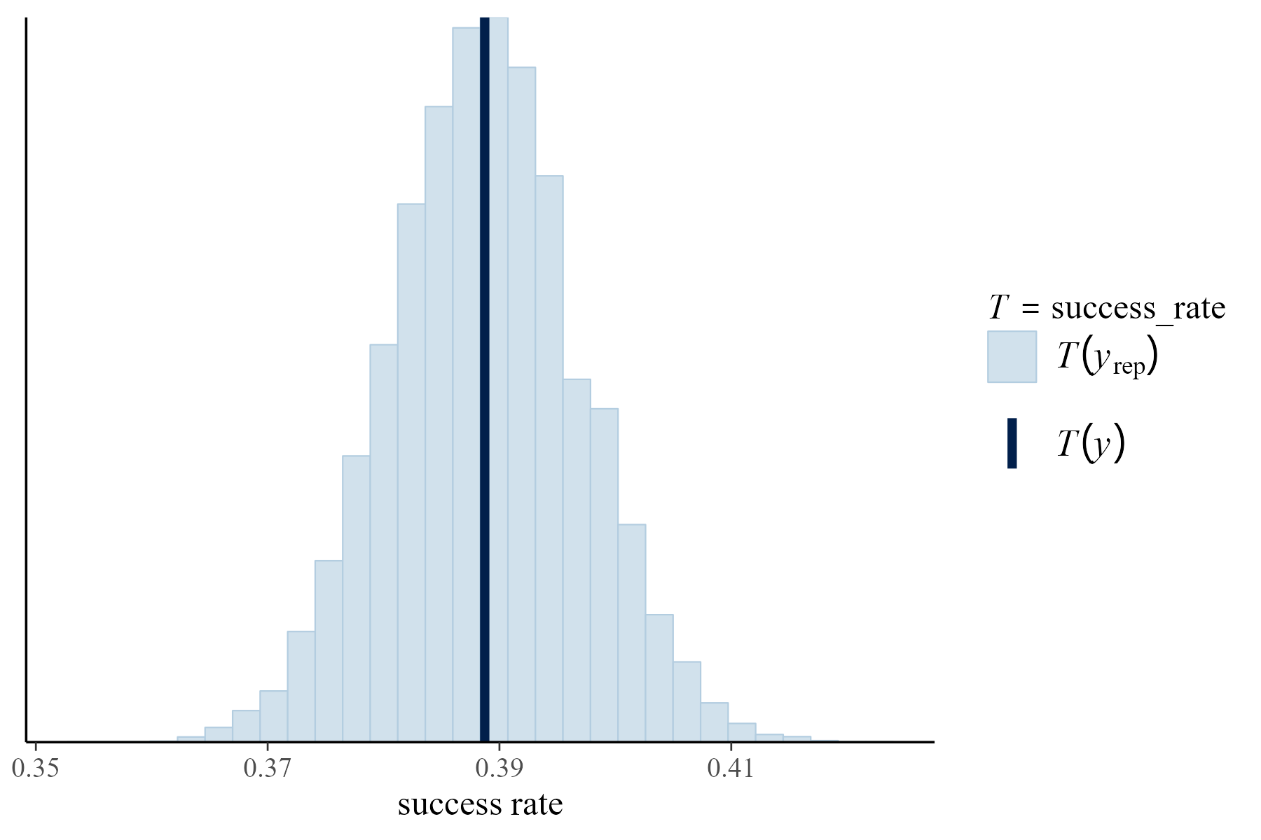
(#fig:18-pp_check_fig)The histogram displays the proportion of climbers that were successful in each of 100 posterior simulated datasets
18.2.2 Posterior analysis
Posterior summaries for our global regression parameters reveal that the likelihood of success decreases with age.
tidy(climb_model,
     effects = "fixed",
     conf.int = TRUE,
     conf.level = 0.80)
Confidence intervals are expressed as the log(odds) to the odds scale, so will be converted to:
\[(e^{-conf.low},e^{-conf.high})=(a,b)\]
On the probability of success scale
\[\pi=\frac{e^{-\beta_0-\beta_1X_1+\beta_2X_2}}{1+e^{-\beta_0-\beta_1X_1+\beta_2X_2}}\]
Results are: both with oxygen and without, the probability of success decreases with age.
climbers %>%
  add_fitted_draws(climb_model, n = 100, re_formula = NA) %>%
  ggplot(aes(x = age, y = success, color = oxygen_used)) +
    geom_line(aes(y = .value, group = paste(oxygen_used, .draw)),
              alpha = 0.1) +
    labs(y = "probability of success")
18.2.3 Posterior classification
New expedition
new_expedition <- data.frame(
  age = c(20, 20, 60, 60), oxygen_used = c(FALSE, TRUE, FALSE, TRUE),
  expedition_id = rep("new", 4))

new_expedition
## age oxygen_used expedition_id
## 1 20 FALSE new
## 2 20 TRUE new
## 3 60 FALSE new
## 4 60 TRUE newPosterior predictions of binary outcome
set.seed(84735)
binary_prediction <- posterior_predict(climb_model, newdata = new_expedition)
# First 3 prediction sets
head(binary_prediction, 3)## 1 2 3 4
## [1,] 0 1 0 1
## [2,] 0 1 0 0
## [3,] 0 1 0 1Summarize the posterior predictions of Y
colMeans(binary_prediction)## 1 2 3 4
## 0.28470 0.80185 0.14755 0.64565