14.5 Two Predictor Variables

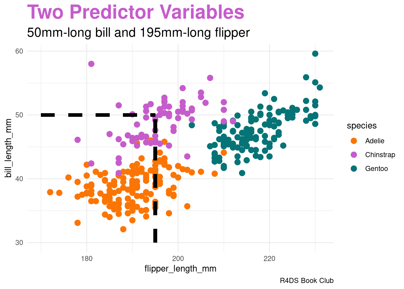
image code

penguins |>
ggplot(aes(x = flipper_length_mm, y = bill_length_mm, 
           color = species)) + 
  geom_point(size = 3) + 
  geom_segment(aes(x = 195, y = 30, xend = 195, yend = 50),
               color = "black", linetype = 2, linewidth = 2) +
  geom_segment(aes(x = 170, y = 50, xend = 195, yend = 50),
               color = "black", linetype = 2, linewidth = 2) +
  labs(title = "<span style = 'color:#c65ccc'>Two Predictor Variables</span>",
       subtitle = "50mm-long bill and 195mm-long flipper",
       caption = "R4DS Book Club") +
  scale_color_manual(values = c(adelie_color, chinstrap_color, gentoo_color)) +
  theme_minimal() +
  theme(plot.title = element_markdown(face = "bold", size = 24),
        plot.subtitle = element_markdown(size = 16))

Generalizing Bayes’ Rule:

$$f(y | x_{2}, x_{3}) = \frac{f(y) \cdot L(y | x_{2}, x_{3})}{\sum_{y'} f(y') \cdot L(y' | x_{2}, x_{3})}$$

Another “naive” assumption of conditionally independent:

$$L(y | x_{2}, x_{3}) = f(x_{2}, x_{3} | y) = f(x_{2} | y) \cdot f(x_{3} | y)$$

• mathematically efficient
• but what about correlation?

# sample statistics of x_3: flipper length
penguins %>% 
  group_by(species) %>% 
  summarize(mean = mean(flipper_length_mm, na.rm = TRUE), 
            sd = sd(flipper_length_mm, na.rm = TRUE))

## # A tibble: 3 × 3
##   species    mean    sd
##   <fct>     <dbl> <dbl>
## 1 Adelie     190.  6.54
## 2 Chinstrap  196.  7.13
## 3 Gentoo     217.  6.48

Likelihoods of a flipper length of 195 mm:

# L(y = A | x_3 = 195) = 0.04554
dnorm(195, mean = 190, sd = 6.54)

# L(y = C | x_3 = 195) = 0.05541
dnorm(195, mean = 196, sd = 7.13)

# L(y = G | x_3 = 195) = 0.0001934
dnorm(195, mean = 217, sd = 6.48)

Total probability:

$$f(x_{2} = 50, x_{3} = 195) = \frac{151}{342} \cdot 0.0000212 \cdot 0.04554 + \frac{68}{342} \cdot 0.112 \cdot 0.05541 + \frac{123}{342} \cdot 0.09317 \cdot 0.0001931 \approx 0.001241$$

Bayes’ Rules:

$$\begin{array}{rcccl} f(y = A | x_{2} = 50, x_{3} = 195) & = & \frac{\frac{151}{342} \cdot 0.0000212 \cdot 0.04554}{0.0001931} & \approx & 0.0003 \\ f(y = C | x_{2} = 50, x_{3} = 195) & = & \frac{\frac{68}{342} \cdot 0.112 \cdot 0.05541}{0.0001931} & \approx & 0.9944 \\ f(y = G | x_{2} = 50, x_{3} = 195) & = & \frac{\frac{123}{342} \cdot 0.09317 \cdot 0.0001931}{0.0001931} & \approx & 0.0052 \\ \end{array}$$

In conclusion, our penguin is almost certainly a Chinstrap.