17.3 Posterior simulation and analysis
# Simulate the posterior !!! new command you can set/update
running_model_1 <- update(running_model_1_prior, prior_PD = FALSE)
##
## SAMPLING FOR MODEL 'continuous' NOW (CHAIN 1).
## Chain 1:
## Chain 1: Gradient evaluation took 5.7e-05 seconds
## Chain 1: 1000 transitions using 10 leapfrog steps per transition would take 0.57 seconds.
## Chain 1: Adjust your expectations accordingly!
## Chain 1:
## Chain 1:
## Chain 1: Iteration: 1 / 10000 [ 0%] (Warmup)
## Chain 1: Iteration: 1000 / 10000 [ 10%] (Warmup)
## Chain 1: Iteration: 2000 / 10000 [ 20%] (Warmup)
## Chain 1: Iteration: 3000 / 10000 [ 30%] (Warmup)
## Chain 1: Iteration: 4000 / 10000 [ 40%] (Warmup)
## Chain 1: Iteration: 5000 / 10000 [ 50%] (Warmup)
## Chain 1: Iteration: 5001 / 10000 [ 50%] (Sampling)
## Chain 1: Iteration: 6000 / 10000 [ 60%] (Sampling)
## Chain 1: Iteration: 7000 / 10000 [ 70%] (Sampling)
## Chain 1: Iteration: 8000 / 10000 [ 80%] (Sampling)
## Chain 1: Iteration: 9000 / 10000 [ 90%] (Sampling)
## Chain 1: Iteration: 10000 / 10000 [100%] (Sampling)
## Chain 1:
## Chain 1: Elapsed Time: 4.479 seconds (Warm-up)
## Chain 1: 3.566 seconds (Sampling)
## Chain 1: 8.045 seconds (Total)
## Chain 1:
##
## SAMPLING FOR MODEL 'continuous' NOW (CHAIN 2).
## Chain 2:
## Chain 2: Gradient evaluation took 3.7e-05 seconds
## Chain 2: 1000 transitions using 10 leapfrog steps per transition would take 0.37 seconds.
## Chain 2: Adjust your expectations accordingly!
## Chain 2:
## Chain 2:
## Chain 2: Iteration: 1 / 10000 [ 0%] (Warmup)
## Chain 2: Iteration: 1000 / 10000 [ 10%] (Warmup)
## Chain 2: Iteration: 2000 / 10000 [ 20%] (Warmup)
## Chain 2: Iteration: 3000 / 10000 [ 30%] (Warmup)
## Chain 2: Iteration: 4000 / 10000 [ 40%] (Warmup)
## Chain 2: Iteration: 5000 / 10000 [ 50%] (Warmup)
## Chain 2: Iteration: 5001 / 10000 [ 50%] (Sampling)
## Chain 2: Iteration: 6000 / 10000 [ 60%] (Sampling)
## Chain 2: Iteration: 7000 / 10000 [ 70%] (Sampling)
## Chain 2: Iteration: 8000 / 10000 [ 80%] (Sampling)
## Chain 2: Iteration: 9000 / 10000 [ 90%] (Sampling)
## Chain 2: Iteration: 10000 / 10000 [100%] (Sampling)
## Chain 2:
## Chain 2: Elapsed Time: 3.76 seconds (Warm-up)
## Chain 2: 3.587 seconds (Sampling)
## Chain 2: 7.347 seconds (Total)
## Chain 2:
##
## SAMPLING FOR MODEL 'continuous' NOW (CHAIN 3).
## Chain 3:
## Chain 3: Gradient evaluation took 3.3e-05 seconds
## Chain 3: 1000 transitions using 10 leapfrog steps per transition would take 0.33 seconds.
## Chain 3: Adjust your expectations accordingly!
## Chain 3:
## Chain 3:
## Chain 3: Iteration: 1 / 10000 [ 0%] (Warmup)
## Chain 3: Iteration: 1000 / 10000 [ 10%] (Warmup)
## Chain 3: Iteration: 2000 / 10000 [ 20%] (Warmup)
## Chain 3: Iteration: 3000 / 10000 [ 30%] (Warmup)
## Chain 3: Iteration: 4000 / 10000 [ 40%] (Warmup)
## Chain 3: Iteration: 5000 / 10000 [ 50%] (Warmup)
## Chain 3: Iteration: 5001 / 10000 [ 50%] (Sampling)
## Chain 3: Iteration: 6000 / 10000 [ 60%] (Sampling)
## Chain 3: Iteration: 7000 / 10000 [ 70%] (Sampling)
## Chain 3: Iteration: 8000 / 10000 [ 80%] (Sampling)
## Chain 3: Iteration: 9000 / 10000 [ 90%] (Sampling)
## Chain 3: Iteration: 10000 / 10000 [100%] (Sampling)
## Chain 3:
## Chain 3: Elapsed Time: 3.786 seconds (Warm-up)
## Chain 3: 3.075 seconds (Sampling)
## Chain 3: 6.861 seconds (Total)
## Chain 3:
##
## SAMPLING FOR MODEL 'continuous' NOW (CHAIN 4).
## Chain 4:
## Chain 4: Gradient evaluation took 3.4e-05 seconds
## Chain 4: 1000 transitions using 10 leapfrog steps per transition would take 0.34 seconds.
## Chain 4: Adjust your expectations accordingly!
## Chain 4:
## Chain 4:
## Chain 4: Iteration: 1 / 10000 [ 0%] (Warmup)
## Chain 4: Iteration: 1000 / 10000 [ 10%] (Warmup)
## Chain 4: Iteration: 2000 / 10000 [ 20%] (Warmup)
## Chain 4: Iteration: 3000 / 10000 [ 30%] (Warmup)
## Chain 4: Iteration: 4000 / 10000 [ 40%] (Warmup)
## Chain 4: Iteration: 5000 / 10000 [ 50%] (Warmup)
## Chain 4: Iteration: 5001 / 10000 [ 50%] (Sampling)
## Chain 4: Iteration: 6000 / 10000 [ 60%] (Sampling)
## Chain 4: Iteration: 7000 / 10000 [ 70%] (Sampling)
## Chain 4: Iteration: 8000 / 10000 [ 80%] (Sampling)
## Chain 4: Iteration: 9000 / 10000 [ 90%] (Sampling)
## Chain 4: Iteration: 10000 / 10000 [100%] (Sampling)
## Chain 4:
## Chain 4: Elapsed Time: 3.641 seconds (Warm-up)
## Chain 4: 3.56 seconds (Sampling)
## Chain 4: 7.201 seconds (Total)
## Chain 4:# Check the prior specifications
prior_summary(running_model_1)## Priors for model 'running_model_1'
## ------
## Intercept (after predictors centered)
## ~ normal(location = 100, scale = 10)
##
## Coefficients
## ~ normal(location = 2.5, scale = 1)
##
## Auxiliary (sigma)
## Specified prior:
## ~ exponential(rate = 1)
## Adjusted prior:
## ~ exponential(rate = 0.072)
##
## Covariance
## ~ decov(reg. = 1, conc. = 1, shape = 1, scale = 1)
## ------
## See help('prior_summary.stanreg') for more details# Markov chain diagnostics
# mcmc_trace(running_model_1)
# mcmc_dens_overlay(running_model_1)
# mcmc_acf(running_model_1)
# neff_ratio(running_model_1)
# rhat(running_model_1)Data output and model:
(Intercept) = \(\beta_0\)
age - \(\beta_1\)
b[(intercept) runner:j] = \(b_{0j} = \beta_{0j} - \beta_0\)
sigma = \(\sigma_y\)
Sigma[runner:(Intercept), (Intercept)] = \(\sigma_0^2\)
17.3.0.1 Posterior analysis of the global relationship
\[\beta_0 + \beta_1X\]
tidy_summary_1 <- tidy(running_model_1, effects = "fixed",
                       conf.int = TRUE, conf.level = 0.80)
tidy_summary_1
## # A tibble: 2 × 5
## term estimate std.error conf.low conf.high
## <chr> <dbl> <dbl> <dbl> <dbl>
## 1 (Intercept) 19.1 12.1 3.58 34.6
## 2 age 1.30 0.217 1.02 1.58So runners are slowing down with age!
17.3.0.2 Posterior analysis of group-specific relationships
\[\beta_{0j} + \beta_1X_{ij} = (\beta_0 + b_{0j}) + \beta_1X_{ij} \]
# Posterior summaries of runner-specific intercepts
# we go from wide to long
runner_summaries_1 <- running_model_1 |>
  spread_draws(`(Intercept)`, b[,runner]) |>
  mutate(runner_intercept = `(Intercept)` + b) |>
  select(-`(Intercept)`, -b) |>
  median_qi(.width = 0.80) |>
  select(runner, runner_intercept, .lower, .upper)
runner_summaries_1
## # A tibble: 36 × 4
## runner runner_intercept .lower .upper
## <chr> <dbl> <dbl> <dbl>
## 1 runner:1 5.23 -10.4 20.9
## 2 runner:10 43.7 27.7 59.5
## 3 runner:11 19.2 3.79 34.8
## 4 runner:12 0.866 -14.7 16.6
## 5 runner:13 10.9 -4.59 26.6
## 6 runner:14 23.7 7.89 39.6
## 7 runner:15 25.6 10.3 41.0
## 8 runner:16 23.3 7.78 38.7
## 9 runner:17 29.2 13.8 44.6
## 10 runner:18 31.2 15.6 46.6
## # ℹ 26 more rowsrunning |>
filter(runner %in% c("4", "5")) |>
add_fitted_draws(running_model_1, n = 100) |>
ggplot(aes(x = age, y = net)) +
geom_line(
aes(y = .value, group = paste(runner, .draw), color = runner),
alpha = 0.1) +
geom_point(aes(color = runner))## Warning: `fitted_draws` and `add_fitted_draws` are deprecated as their names were confusing.
## - Use [add_]epred_draws() to get the expectation of the posterior predictive.
## - Use [add_]linpred_draws() to get the distribution of the linear predictor.
## - For example, you used [add_]fitted_draws(..., scale = "response"), which
## means you most likely want [add_]epred_draws(...).
## NOTE: When updating to the new functions, note that the `model` parameter is now
## named `object` and the `n` parameter is now named `ndraws`.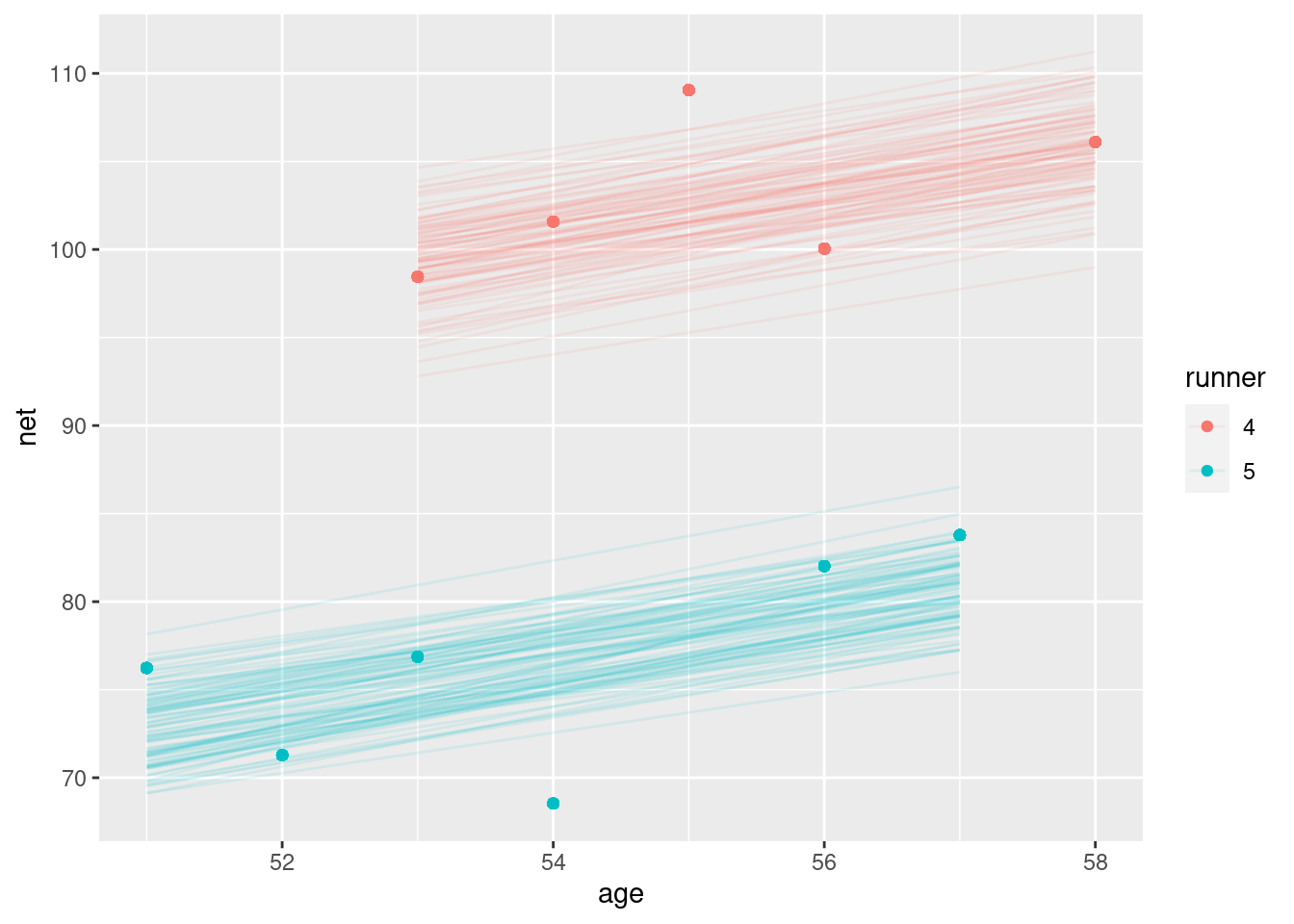
17.3.0.3 Posterior analysis of within- and between group variability
tidy_sigma <- tidy(running_model_1, effects = "ran_pars")
tidy_sigma
## # A tibble: 2 × 3
## term group estimate
## <chr> <chr> <dbl>
## 1 sd_(Intercept).runner runner 13.3
## 2 sd_Observation.Residual Residual 5.26sigma_0 <- tidy_sigma[1,3]
sigma_y <- tidy_sigma[2,3]
sigma_0^2 / (sigma_0^2 + sigma_y^2) # between## estimate
## 1 0.8648491sigma_y^2 / (sigma_0^2 + sigma_y^2) # within## estimate
## 1 0.1351509