5.12 Gamma-Poisson conjugate family 8/8

Now need a posterior!

\[ \tau|\overrightarrow{y} \sim Gamma(s + \sum y_i, r +n) \] We have: Gamma(10,2) and as data: \(\overrightarrow{y} = (6 + 2 + 2+ 1 )\) , \(n = 4\)

\[\sum_{i = 1}^{4} = 6 + 2 + 2 + 1 =11\]

\[\overline{y} = \frac{\sum_{i = 1}^{4}}{4} = 2.75\]

\[L(\tau|\overrightarrow{y}) = \frac{\tau^ye^{-n\tau}}{y!}\]

\[L(\tau|\overrightarrow{y}) = \frac{\tau^{11}e^{-4\tau}}{6!2!2!1!} \propto \tau^{11}e^{-4\tau}\]

bayesrules::plot_poisson_likelihood(y = c(6, 2, 2, 1), lambda_upper_bound = 10)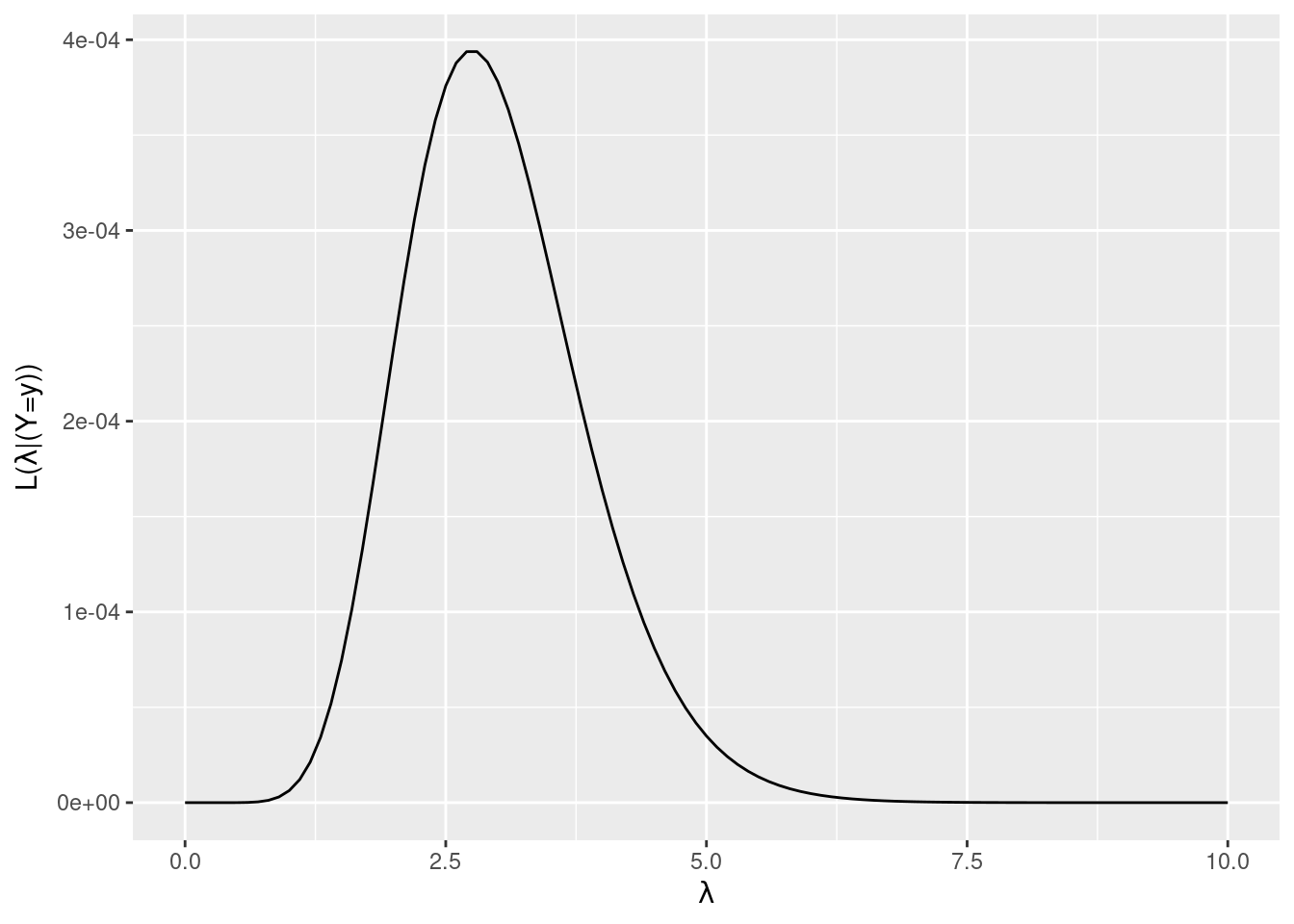

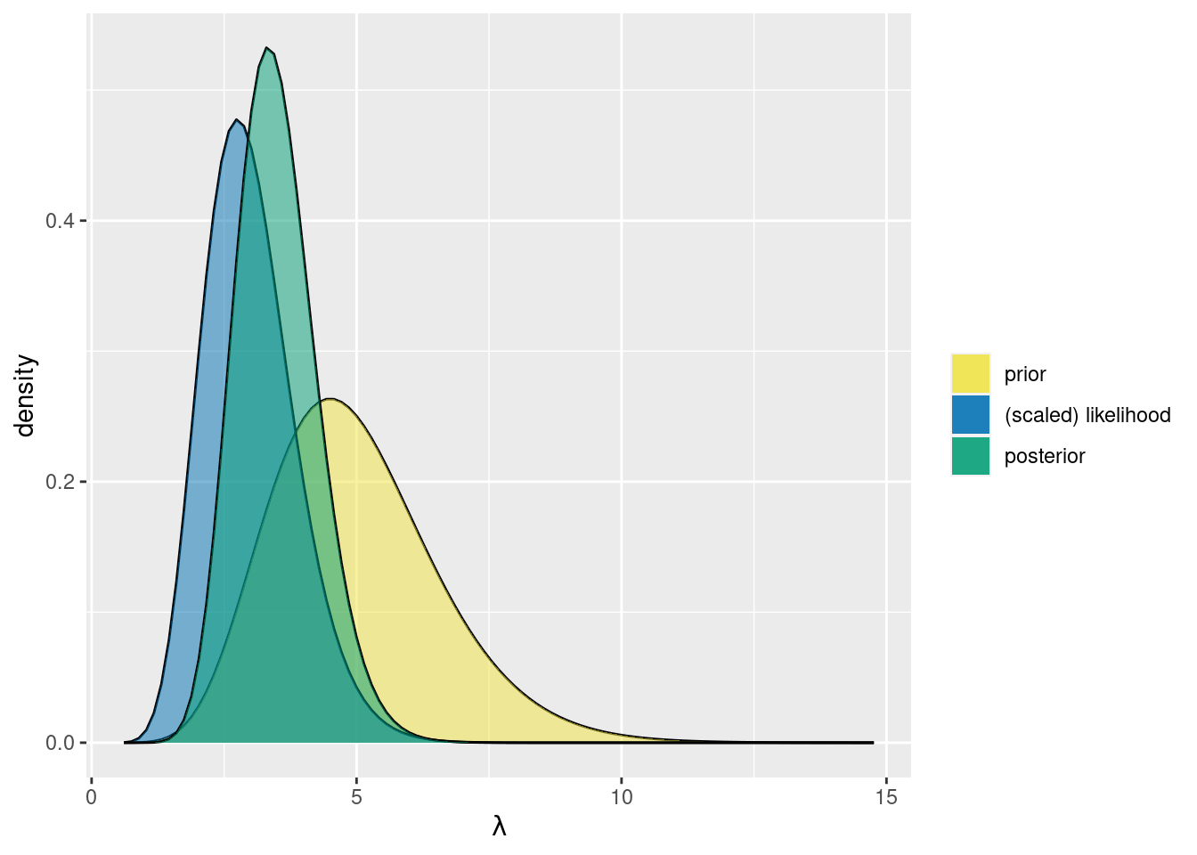
We have prior, data, likelihood -> posterior

\[Gamma(10, 2) \longrightarrow Gamma(s + \sum y_i, r +n)\]

\[\tau|\overrightarrow{y} \sim Gamma(21, 6) \]

bayesrules::plot_gamma_poisson(shape = 10, rate = 2, sum_y = 11, n = 4)