16.4 Building the hierarchical model
16.4.1 The hierarchy
Layer 1: \(Y_{ij} | \mu_j , \sigma_y\) how song popularity varies WITHIN artist \(j\)
Layer 2: \(\mu_{j}|\mu, \sigma_\mu\) how typical popularity \(\mu_{j}\) varies BETWEEN artists
Layer 3: \(\mu, \sigma_y, \sigma_{\mu}\) prior models for shared global parameters
(order do not necessarily matter)
Layer 1:
\[Y_{ij}|\mu_j, \sigma_j \sim N(\mu_j, \sigma_y^2)\]
\(\mu_j\) mean song popularity for artist j
\(\sigma_y\) within group variability sd in popularity from song to song within each artist
-> if we stop here we have a “no pooled”
Layer 2:
\[\mu_{j}|\mu_{j}. \sigma_\mu \overset{ind}{\sim} N(\mu, \sigma_\mu^2)\] \(\mu\) global average: the means popularity ratings for the most average artist
\(\sigma_{u}\) \(between-group variability\), the standard deviation in mean popularity \(μj\) from artist to artist.
#Normal is not too bad
ggplot(artist_means, aes(x = popularity)) +
  geom_density()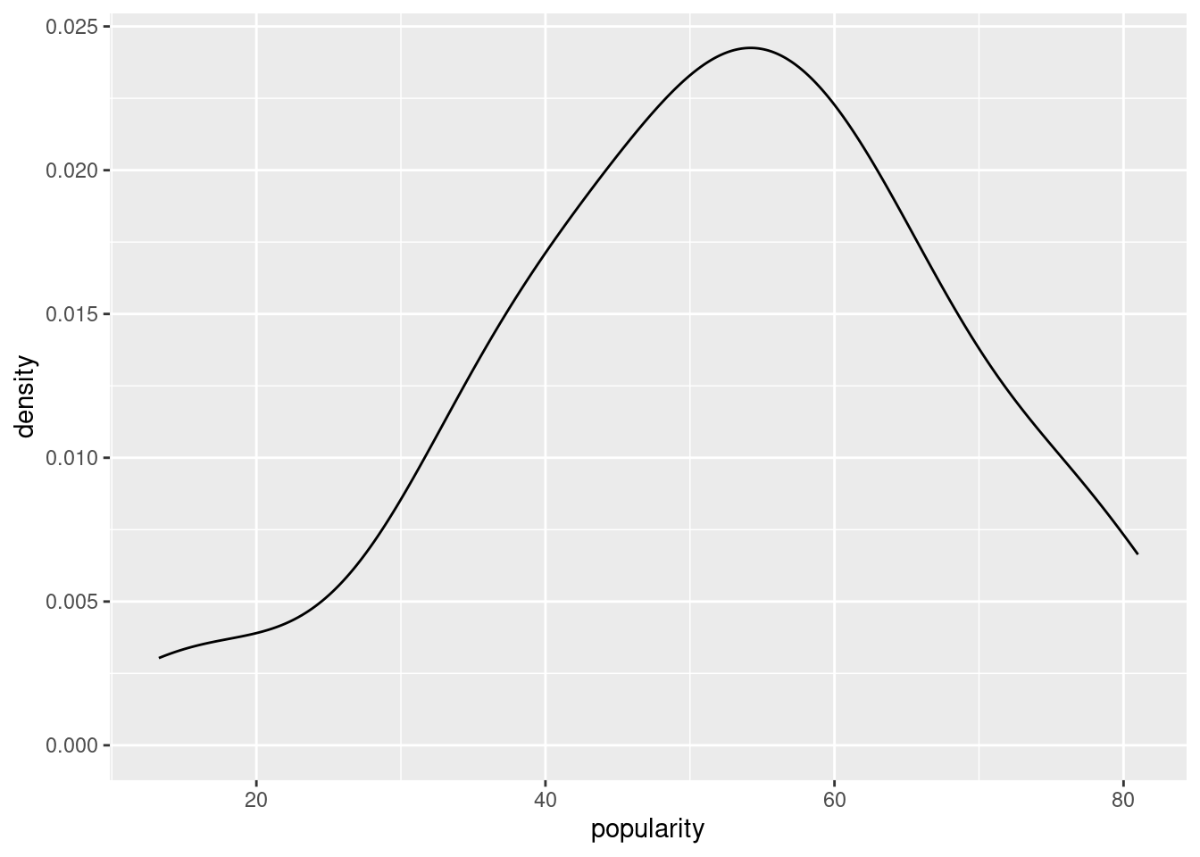
Layer 3 : Priors
\[\mu \sim N(50, 52^2)\] (this 52 ???)
\[\sigma_y \sim Exp(0.048) \]
\[ \sigma \sim Exp(1)\]

@realHollanders
This is a one way analyis of variance (ANOVA)
An other way to think about it:
\[Y_{ij}|\mu_j, \sigma_j \sim N(\mu_j, \sigma_y^2) \quad with \quad \mu_j = \mu +b_j\]
\[b_j | \sigma_\mu \overset{ind}{\sim} N(0, \sigma_\mu^2) \]
Example: if \(\mu\) = 55 and \(\mu_j\) = 65 \(b_j\) = 10
16.4.2 within- vs -between-group variability
Before we analyse just one source of variability (the individual level), now we have two sources (\(\sigma_\mu, \sigma_y\)). The first one is the sqrt(variance) within the group (song of an artist) and the second is the sqrt(variance) between group.
The total variance is :
\[Var(Y_{ij} = \sigma²_y + \sigma^2_u) \] Other way of thinking about is:
\(\frac{\sigma^2_y}{\sigma^2_\mu + \sigma^2_y}\) proportion of total variance explained by difference within each group
\(\frac{\sigma^2_\mu}{\sigma^2_\mu + \sigma^2_y}\) proportion of total variance explained by difference between groups
You have correlation in song popularity of the same artist (within group). And assuming each groups are independant we get:
\[Cor(Y_{ij}, Y_{kj}) = \frac{\sigma^2_\mu}{\sigma^2_\mu + \sigma^2_y}\] ## Posterior analysis
16.4.3 Posterior simulation
47 parameters:
- 44 artists specific parameters (\(\mu_{j}\))
- 3 global parameters (\(\mu, \sigma_j, sigma_\mu\))
spotify_hierarchical <- stan_glmer(
  popularity ~ (1 | artist), # this  is the part that tell that artist is a group not a predictor
  data = spotify, family = gaussian,
  prior_intercept = normal(50, 2.5, autoscale = TRUE),
  prior_aux = exponential(1, autoscale = TRUE),
  prior_covariance = decov(reg = 1, conc = 1, shape = 1, scale = 1), # stuff we will learn chapter 17 suppose to be equivalent to Exp(1)
  chains = 4, iter = 5000*2, seed = 84735)
# Confirm the prior tunings
prior_summary(spotify_hierarchical)## Priors for model 'spotify_hierarchical'
## ------
## Intercept (after predictors centered)
## Specified prior:
## ~ normal(location = 50, scale = 2.5)
## Adjusted prior:
## ~ normal(location = 50, scale = 52)
##
## Auxiliary (sigma)
## Specified prior:
## ~ exponential(rate = 1)
## Adjusted prior:
## ~ exponential(rate = 0.048)
##
## Covariance
## ~ decov(reg. = 1, conc. = 1, shape = 1, scale = 1)
## ------
## See help('prior_summary.stanreg') for more detailsWe need to check the success of MCMC (saving you time here)
bayesplot::pp_check(spotify_hierarchical) + xlab("popularity")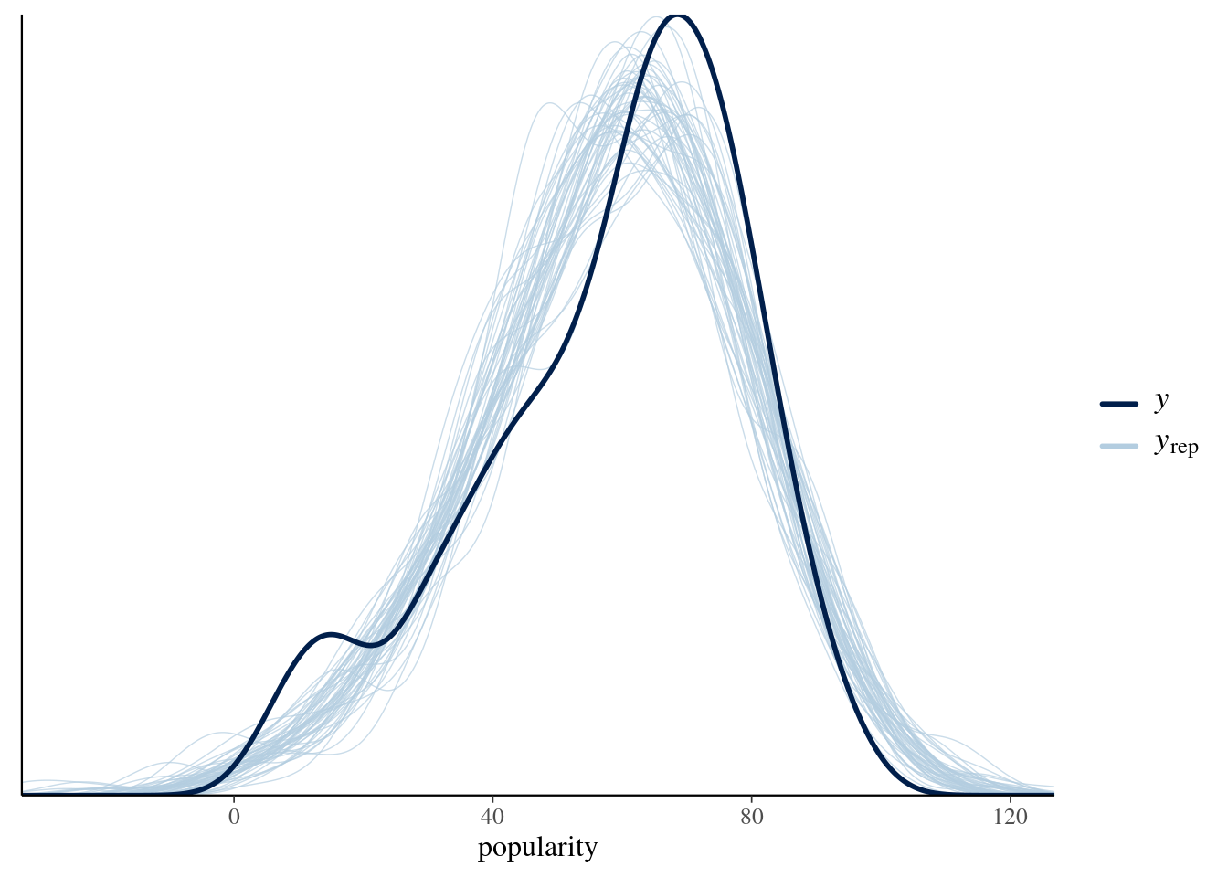
Let inspect our simulation:
spotify_hierarchical_df <- as.data.frame(spotify_hierarchical)
dim(spotify_hierarchical_df)
## [1] 20000 4716.4.4 Posterior analysis of global parameters
- \(\mu = (intercept)\)
- \(\sigma_y = sigma\)
- \(\sigma_\mu² = Sigma[artist:(intercep),(Intercept)]\) Attention! here this is the variance
tidy(spotify_hierarchical, effects = "fixed" # for getting global
     , conf.int = TRUE, conf.level = 0.80)
## # A tibble: 1 × 5
## term estimate std.error conf.low conf.high
## <chr> <dbl> <dbl> <dbl> <dbl>
## 1 (Intercept) 52.5 2.44 49.3 55.6tidy(spotify_hierarchical,
effects = "ran_pars") # PARameters and RANdomness or variability)## # A tibble: 2 × 3
## term group estimate
## <chr> <chr> <dbl>
## 1 sd_(Intercept).artist artist 15.2
## 2 sd_Observation.Residual Residual 14.0An other way:
15.1^2 / (15.1^2 + 14.0^2) # sigma_mu^2 / sigma_mu^2 + sigma_y^2 ## [1] 0.537746814.0^2 / (15.1^2 + 14.0^2) # sigma_y^2 / sigma_mu^2 + sigma_y^2## [1] 0.462253216.4.5 posterior analysis of group specific
If you recall that \(\mu_j = \mu + b_{j}\)
We have \(\mu\) and \(b_j\) (check spotify_hierarchical_df)
 # RANdom Values
artist_summary <- tidy(spotify_hierarchical, effects = "ran_vals"
                       , conf.int = TRUE, conf.level = 0.80)

# Check out the results for the first & last 2 artists
# 80% intervall
# this produce a summary
artist_summary %>%
  select(level, conf.low, conf.high) %>%
  slice(1:2, 43:44)
## # A tibble: 4 × 3
## level conf.low conf.high
## <chr> <dbl> <dbl>
## 1 Mia_X -40.8 -23.2
## 2 Chris_Goldarg -39.4 -26.8
## 3 Lil_Skies 11.0 30.2
## 4 Camilo 19.4 32.4dim(artist_summary)## [1] 44 7Other way: combining simulations to simulate posterior of \(\mu_j\)
\[\mu_j = \mu + b_{j} = (Intercept) + b[(Intercept) \quad artist:j]\]
artist_chains <- spotify_hierarchical |>
  spread_draws(`(Intercept)`, b[,artist]) |>
  mutate(mu_j = `(Intercept)` + b)

dim(artist_chains)
## [1] 880000 7artist_chains |>
select(artist, `(Intercept)`, b, mu_j) |>
head(4)## # A tibble: 4 × 4
## # Groups: artist [4]
## artist `(Intercept)` b mu_j
## <chr> <dbl> <dbl> <dbl>
## 1 artist:Alok 49.9 12.6 62.5
## 2 artist:Atlas_Genius 49.9 -12.8 37.1
## 3 artist:Au/Ra 49.9 10.7 60.6
## 4 artist:Beyoncé 49.9 22.9 72.8# Get posterior summaries for mu_j
artist_summary_scaled <- artist_chains |>
select(-`(Intercept)`, -b) |>
mean_qi(.width = 0.80) |>
mutate(artist = fct_reorder(artist, mu_j))
# Check out the results
artist_summary_scaled |>
select(artist, mu_j, .lower, .upper) |>
head(4)## # A tibble: 4 × 4
## artist mu_j .lower .upper
## <fct> <dbl> <dbl> <dbl>
## 1 artist:Alok 64.3 60.2 68.4
## 2 artist:Atlas_Genius 47.1 38.9 55.1
## 3 artist:Au/Ra 59.5 52.2 66.9
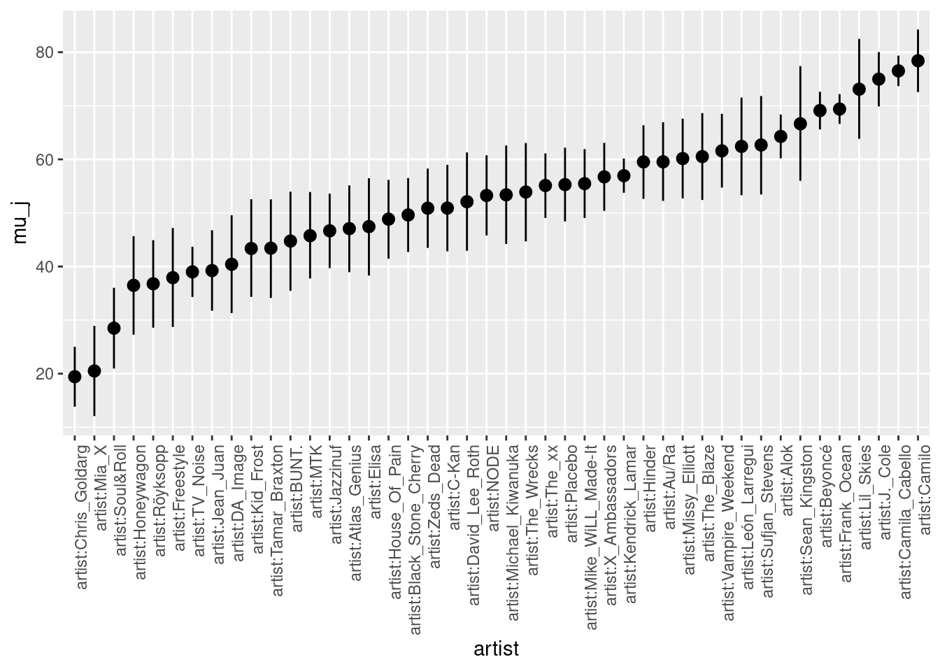
## 4 artist:BUNT. 44.8 35.5 54.0ggplot(artist_summary_scaled,
aes(x = artist, y = mu_j, ymin = .lower, ymax = .upper)) +
geom_pointrange() +
xaxis_text(angle = 90, hjust = 1)