4.4 Striking a balance between the prior and data
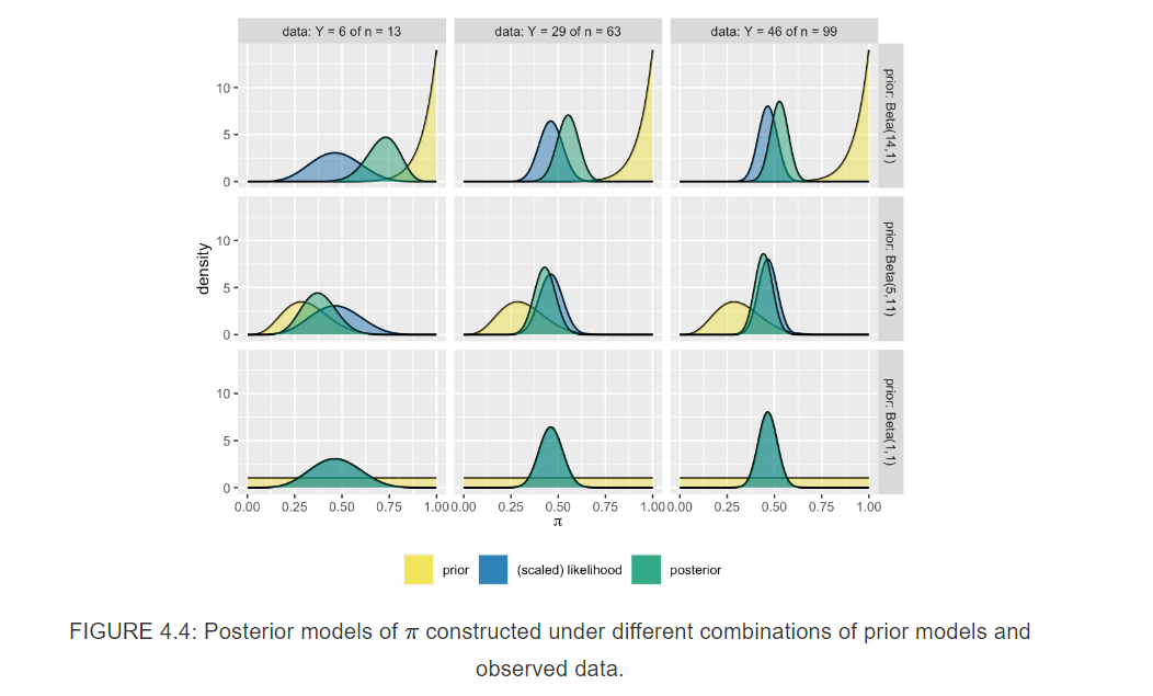
The grid of plots illustrates the balance that the posterior model strikes between the prior and data. Each row corresponds to a unique prior model and each column to a unique set of data.
The likelihood’s insistence and, correspondingly, the data’s influence over the posterior increase with sample size n.
The influence of our prior understanding diminishes as we amass new data. Further, the rate at which the posterior balance tips in favor of the data depends upon the prior.
Naturally, the more informative the prior, the greater its influence on the posterior.
KEY UNDERSTANDING: no matter the strength of and discrepancies among their prior understanding of \(\pi\), three analysts will come to a common posterior understanding in light of strong data.
# Plot the Beta-Binomial model
plot_beta_binomial(alpha = 5, beta =11, y = 50, n = 99)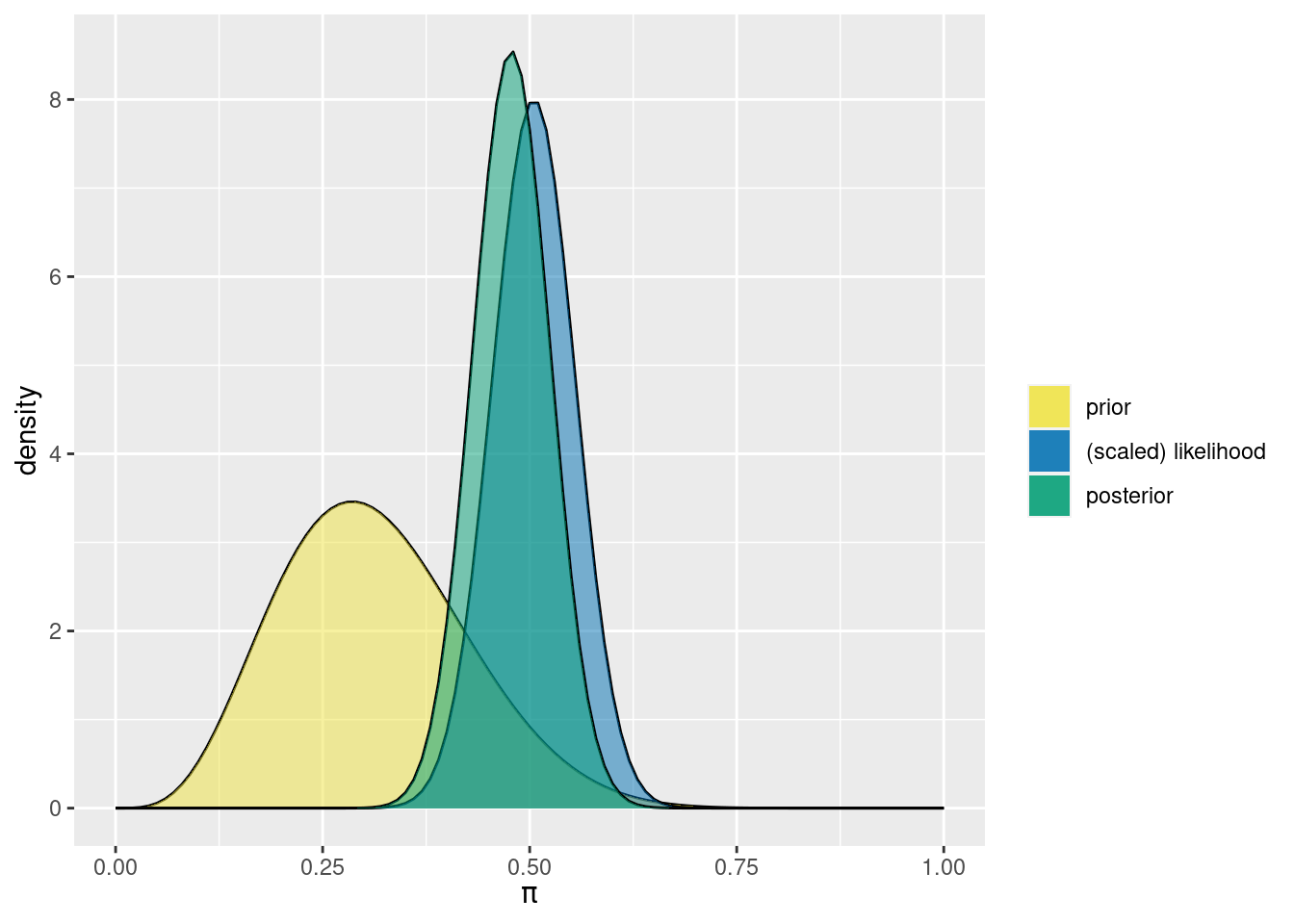
# Obtain numerical summaries of the Beta-Binomial model
summarize_beta_binomial(alpha = 5, beta = 11, y = 50, n = 99) %>%
  gt() %>%
  fmt_number(columns = c(mean, mode, var, sd),
             decimals = 2) %>%
tab_options(column_labels.font.weight = 'bold')| model | alpha | beta | mean | mode | var | sd |
|---|---|---|---|---|---|---|
| prior | 5 | 11 | 0.31 | 0.29 | 0.01 | 0.11 |
| posterior | 55 | 60 | 0.48 | 0.48 | 0.00 | 0.05 |