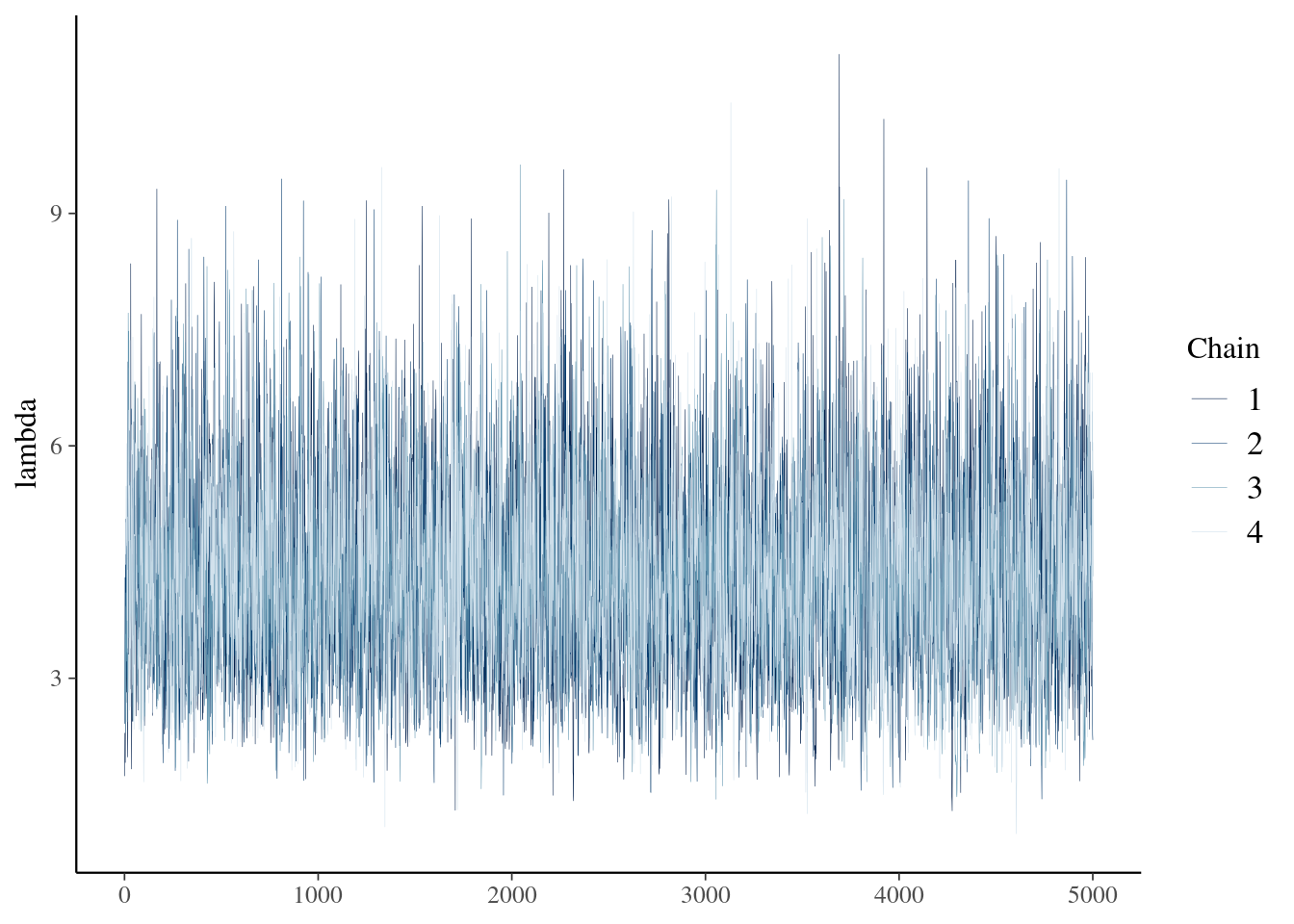
6.8 Markov chain diagnostics

How do we know if a MCMC process is “good”?

• Primary tools:
  • Trace plots
  • Effective sample size
  • Autocorrelation
  • R-hat
• With trace plots, look for good mixing and compare parallel chains.

• Effective sample size takes into account the correlation between samples. (best if > 10% of actual samples)

neff_ratio(bb_sim, pars = c("pi"))

## [1] 0.3609688

# Density plots of individual chains
mcmc_dens_overlay(bb_sim, pars = "pi") + 
  ylab("density")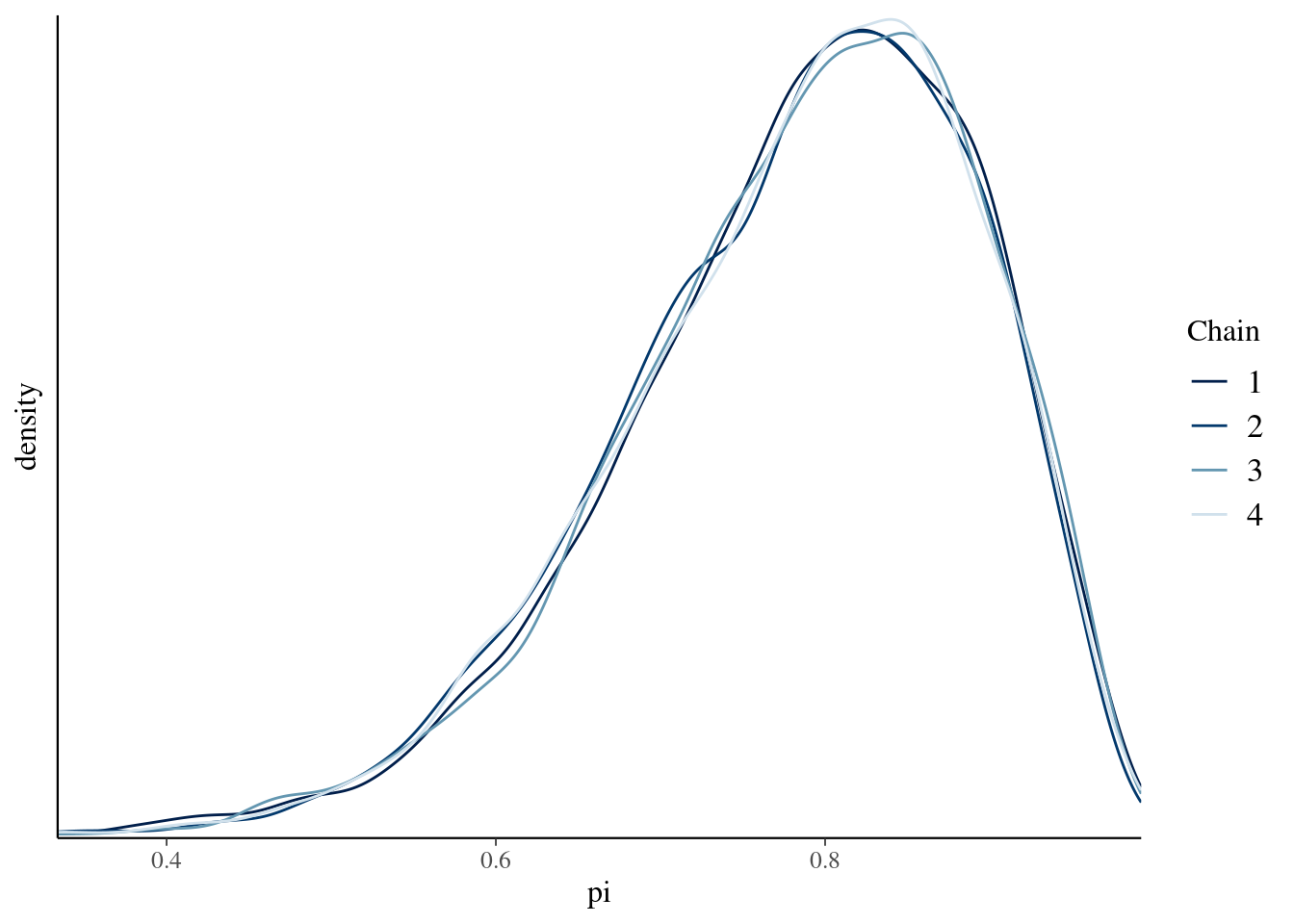

• Autocorrelation measures the correlation between pairs of Markov chain values that are Lag “steps” apart

mcmc_acf(bb_sim, pars = "pi")

## Warning: The `facets` argument of `facet_grid()` is deprecated as of ggplot2 2.2.0.
## ℹ Please use the `rows` argument instead.
## ℹ The deprecated feature was likely used in the bayesplot package.
##   Please report the issue at <https://github.com/stan-dev/bayesplot/issues/>.
## This warning is displayed once every 8 hours.
## Call `lifecycle::last_lifecycle_warnings()` to see where this warning was
## generated.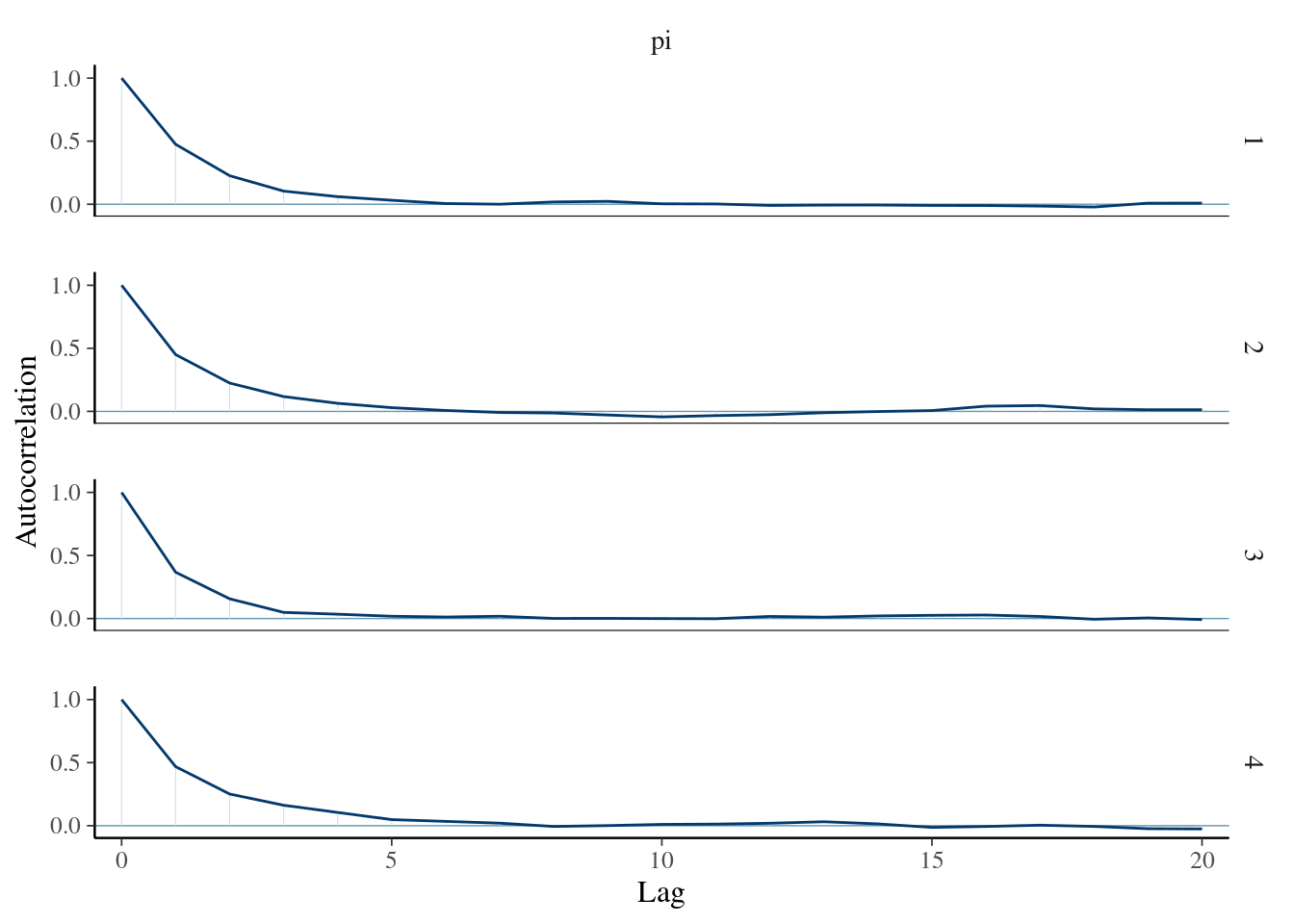

• R-hat is the ratio of the variability between chains to the variability within chains.

  • R-hat \(\approx\) 1 is ideal
  • R-hat > 1.05 is cause for concern.

rhat(bb_sim, pars="pi")

## [1] 1.000064