17.4 Hierarchical model with varying intercepts & slopes
ggplot(running, aes(x = age, y = net, group = runner)) +
  geom_smooth(method = "lm", se = FALSE, size = 0.5)
## `geom_smooth()` using formula = 'y ~ x'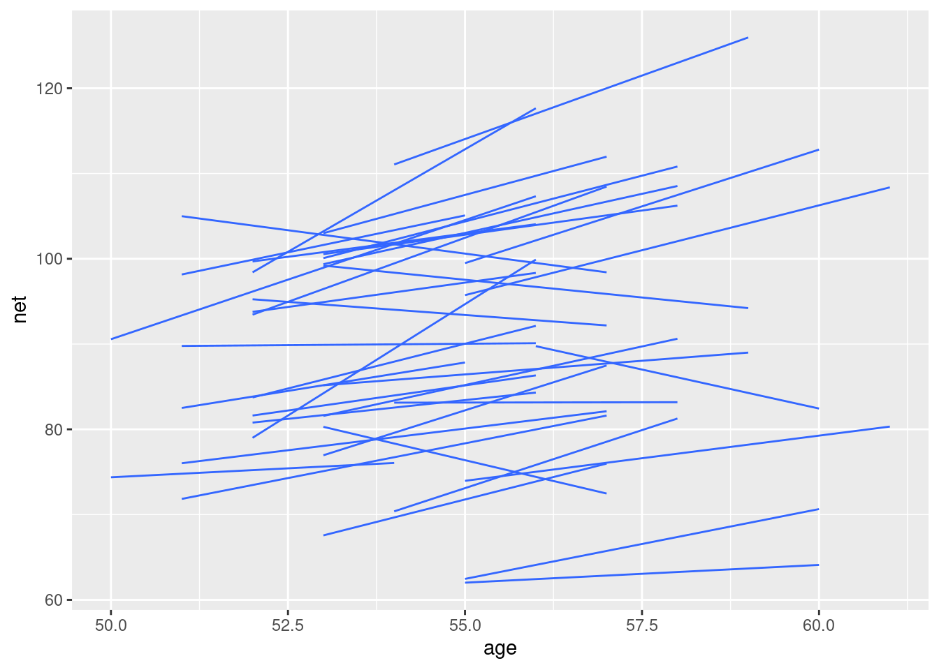
Quiz!

source:thebrain187
How can we modify our random intercepts models to recognize that the rate at which running time change with age might vary from runner to runner?
17.4.1 Model building
\[Y_{ij} | \beta_{0j}, \beta_{1j}, \sigma_y \sim N(\mu_{ij}, \sigma_y^2)\]
\[\mu_{ij} = \beta_{0j} + \beta_{1j}X_{ij}\]
\[\beta_{0j} | \beta_{0}, \sigma_0 \sim N(\beta_0, \sigma_0^2)\]
\[\beta_{1j} | \beta_{1}, \sigma_1 \sim N(\beta_1, \sigma_1^2)\] But \(\beta_{0j}\) and \(\beta_{1j}\) are correlated for runner j. Let \(\rho \in [-1,1]\) represent the correlation between \(\beta_{0j}\) and \(\beta_(1j)\). We will need to do a joint Normal model of both:
\[\begin{pmatrix} \beta_{0j} \\ \beta_{1j} \end{pmatrix} | \beta_0, \beta_1, \sigma_0, \sigma_1 \sim N \begin{pmatrix}\begin{pmatrix} \beta_0 \\ \beta_1 \end{pmatrix}, \Sigma \end{pmatrix}\]
\[ \Sigma = \begin{pmatrix} \sigma_0² & \rho\sigma_0\sigma_1 \\ \rho\sigma_0\sigma_1 & \sigma_1^2 \end{pmatrix} \]
\(\Sigma\) is our covariance matrix
Let me google it for you:
\[\rho(X,Y) = \frac{Cov(X,Y)}{\sigma_X\sigma_y} \in [-1, 1]\]
Examples:
strong negative correlation between \(\beta_{0j}\) and \(\beta_{1j}\) with small intercept: smaller you start higher you go
strong positive correlation with small intercept : smaller you start lower you go
no correlation : X and Y do their life
Quiz!
- \(\beta_{0j}\) and \(\beta_{1j}\) are negatively correlated:
- Runners that start out slower (i.e., with a higher baseline), also tend to slow down at a more rapid rate.
- The rate at which runners slow down over time isn’t associated with how fast they start out.
- Runners that start out faster (i.e., with a lower baseline), tend to slow down at a more rapid rate.
- \(\beta_{0j}\) and \(\beta_{1j}\) are positively correlated:
If \(\sigma_1 = 0\), age will not differ group to group we are back to the random intercepts model.
But how do we get our Joint prior model?
We are using a decomposition of covariance model and the function decov() (rememver the prior_covariance = decov(reg = 1, conc = 1, shape = 1, scale = 1) in our stan_glmer call)
We can decompose our matrix in 3 components:
\[R = \begin{pmatrix} 1 & \rho \\ \rho & 1 \end{pmatrix}\]
\[ \tau = \sqrt{\sigma^2_0 + \sigma^2_1}\]
\[ \pi = \begin{pmatrix} \pi_0 \\ \pi_1 \end{pmatrix} = \begin{pmatrix}\frac{\sigma_0^2}{\sigma_0^2 + \sigma_1^2} \\ \frac{\sigma_1^2}{\sigma_0^2 + \sigma_1^2} \end{pmatrix}\]
\[R \sim LKJ(\eta)\]
Lewandowski-Kurowicka-Joe (LKJ) distribution with \(\eta\) as **regularization hyperparameter
if \(\eta < 1\) prior with strong correlation unsure of postive or negative
if \(\eta = 1\) flat prior between - 1 and 1
if \(\eta > 1\) prior indicating low correlation
For \(\tau\) we can use a Gamma prior (or here the exponential special case). It use two parameters : shape and scale.
Finaly for \(\pi\) we know that the sum of them will be one (remember they are the relative proportion of the variability between group). This means we will be able to use a symmetric Dirichlet(\(2, \delta\)). \(\delta\) is called a concentration hyperparameter.
In this case with two group it can be define as a Beta distribution with both (\(\delta\)).
if \(\delta < 1\) more prior on \(\pi_0\) on 0, 1 -> either a lot of few of the variability between group is explained with intercept
\(\delta = 1\) flat prior on \(\pi_0\) variability of the intercept can explain from 0 to all the variability between groups
\(\delta > 1\) our prior is that around half of the variability between group is explained by differences in intercepts and rest with slopes.
To sum it up when we use rstanarm decov():
reg = 1is for \(R \sim LKJ(1)\)shape = 1 , scale = 1is for \(\tau \sim Gamma(1,1)\) or \(Exp(1)\)conc = 1is for \(Dirichlet(2,1)\) (two parameters with \(\delta = 1\))
17.4.2 Posterior simulation and anlysis
running_model_2 <- stan_glmer(
  net ~ age + (age | runner),
  data = running, family = gaussian,
  prior_intercept = normal(100, 10),
  prior = normal(2.5, 1),
  prior_aux = exponential(1, autoscale = TRUE),
  prior_covariance = decov(reg = 1, conc = 1, shape = 1, scale = 1),
  chains = 4, iter = 5000*2, seed = 84735, adapt_delta = 0.99999 # change here
)
Now we have 78 parameters (36 for intercepts / 36 age coefficient and 6 global parameters) !

My poor laptop have done it in 33 minutes!
17.4.2.1 Global / Group specific parameters :
\[\beta_0 + \beta_1 X \]
# Quick summary of global regression parameters
tidy(running_model_2, effects = "fixed", conf.int = TRUE, conf.level = 0.80)
# A tibble: 2 x 5
  term        estimate std.error conf.low conf.high
  <chr>          <dbl>     <dbl>    <dbl>     <dbl>
1 (Intercept)    18.5     11.6       3.61     33.6
2 age             1.32     0.217     1.04      1.59
We need to move the MCMC simulations result into a friendlier objet:
# str(running_model_2) try it!runner_chains_2 <- running_model_2 |>
spread_draws(`(Intercept)`, b[term, runner], `age`) |>
pivot_wider(names_from = term, names_glue = "b_{term}",
values_from = b) |>
mutate(runner_intercept = `(Intercept)` + `b_(Intercept)`,
runner_age = age + b_age)
dim(runner_chains_2)We need to summarize a bit:
runner_summaries_2 <- runner_chains_2 |>
  group_by(runner) |>
  summarize(runner_intercept = median(runner_intercept),
            runner_age = median(runner_age))

# Check it out
head(runner_summaries_2, 3)
saveRDS(runner_summaries_2, "data/ch17/runner_summaries_2")
runner_summaries_2 <- readRDS("data/ch17/runner_summaries_2")
ggplot(running, aes(y = net, x = age, group = runner)) +
geom_abline(data = runner_summaries_2, color = "gray",
aes(intercept = runner_intercept, slope = runner_age)) +
lims(x = c(50, 61), y = c(50, 135))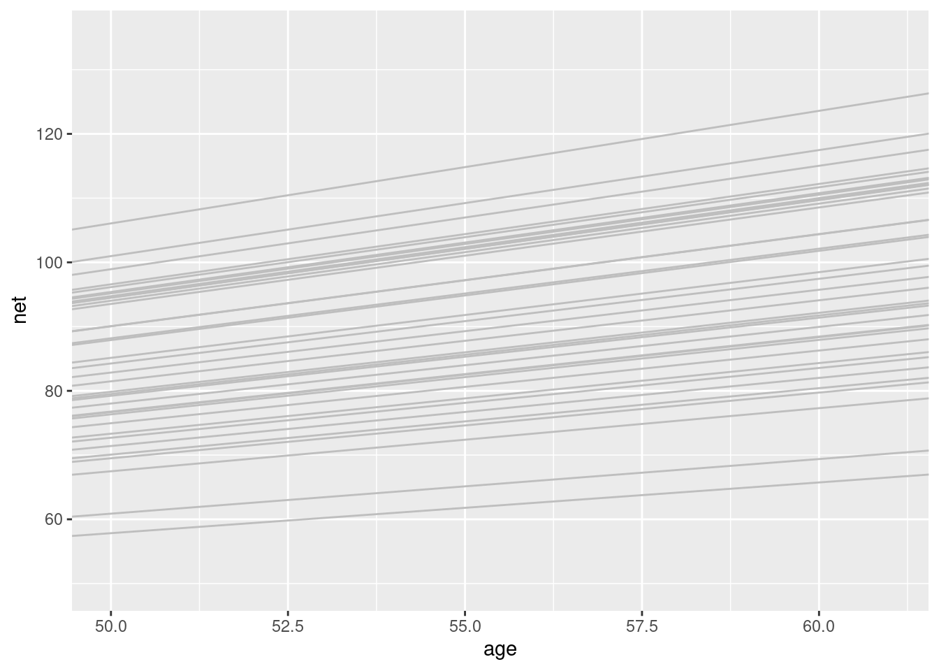
They slopes differ but no so much -> shrinkage the model is still trying to balance between a complete pooled models and a no pooled one (see fig 17.16).
17.4.2.2 Within- and between-group variability
is it worth it ?
tidy(running_model_2, effects = "ran_pars")
# A tibble: 4 x 3
  term                       group    estimate
  <chr>                      <chr>       <dbl>
1 sd_(Intercept).runner      runner     1.34
2 sd_age.runner              runner     0.251
3 cor_(Intercept).age.runner runner    -0.0955
4 sd_Observation.Residual    Residual   5.17
We had 5.25 as \(\sigma_y\) before, We have very slight correlation between \(\beta_0j\) and \(\beta_1j\).