18.3 Hierarchical Poisson & Negative Binomial regression
# Load data
data(airbnb)

# Number of listings
nrow(airbnb)
## [1] 1561# Number of neighborhoods
airbnb %>%
summarize(nlevels(neighborhood))## nlevels(neighborhood)
## 1 43 # nlevels(neighborhood)18.3.1 Model building & simulation
ggplot(airbnb, aes(x = reviews)) +
  geom_histogram(color = "white", breaks = seq(0, 200, by = 10))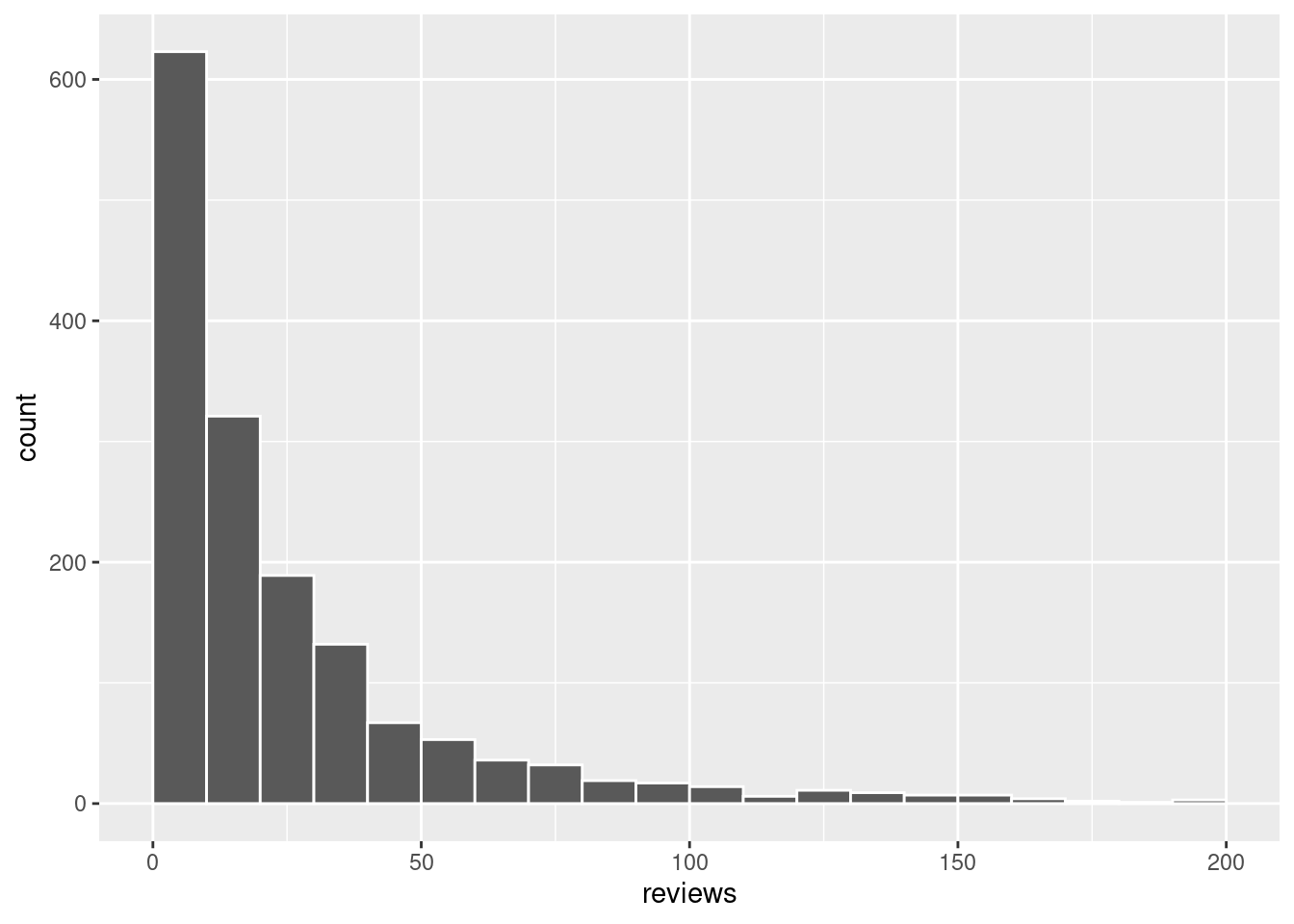
ggplot(airbnb, aes(y = reviews, x = rating)) +
  geom_jitter()
ggplot(airbnb, aes(y = reviews, x = room_type)) +
  geom_violin()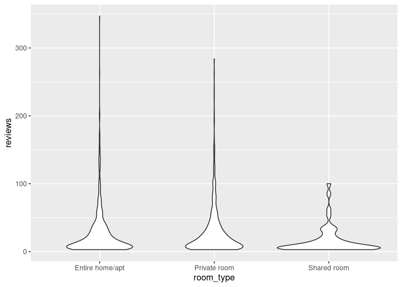
airbnb %>%
  filter(neighborhood %in%
           c("Albany Park", "East Garfield Park", "The Loop")) %>%
  ggplot(aes(y = reviews, x = rating, color = room_type)) +
    geom_jitter() +
    facet_wrap(~ neighborhood)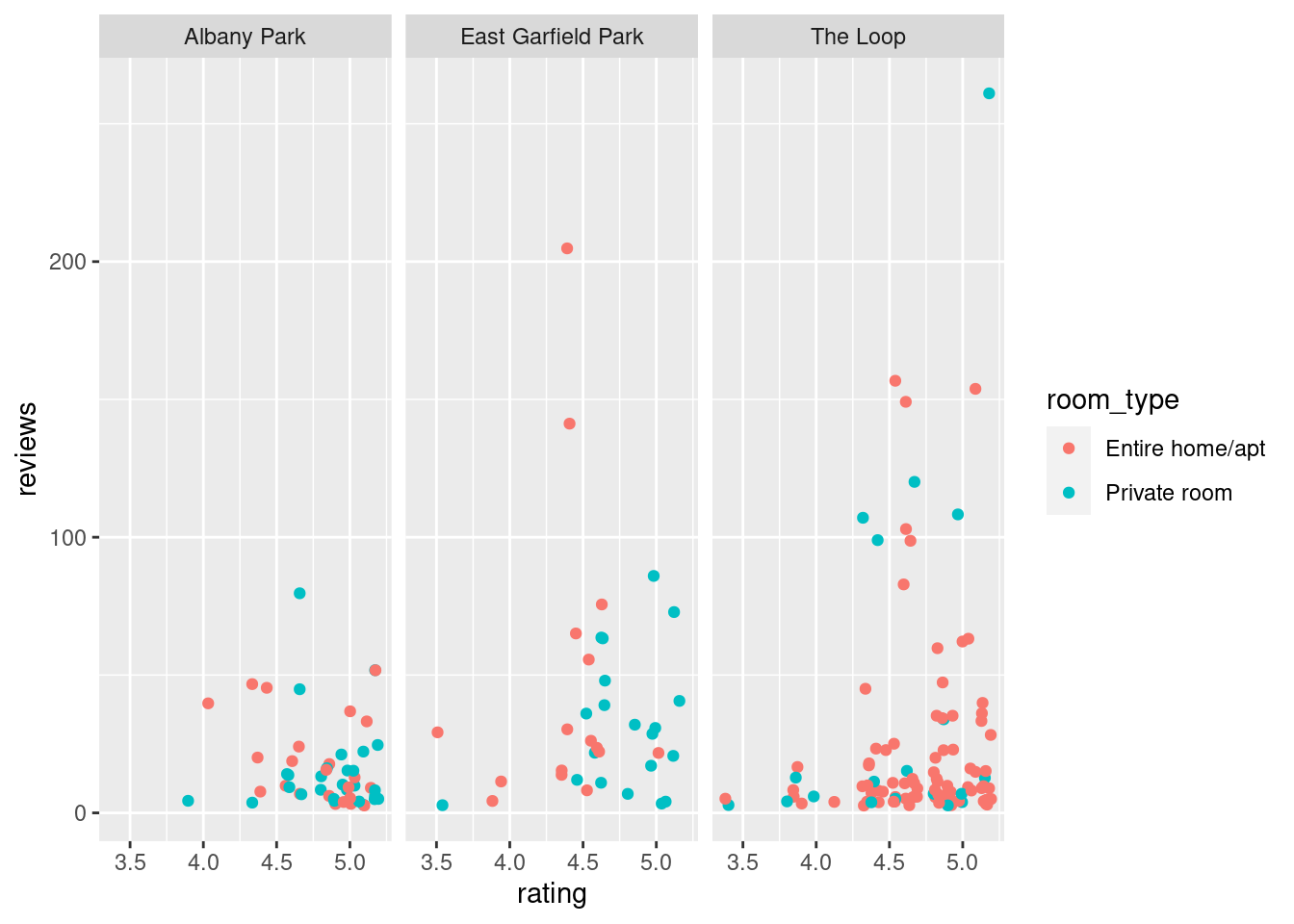
airbnb_model_1 <- stan_glmer(
  reviews ~ rating + room_type + (1 | neighborhood),
  data = airbnb, family = poisson,
  prior_intercept = normal(3, 2.5, autoscale = TRUE),
  prior = normal(0, 2.5, autoscale = TRUE),
  prior_covariance = decov(reg = 1, conc = 1, shape = 1, scale = 1),
  chains = 4, iter = 5000*2, seed = 84735
)pp_check(airbnb_model_1) +
xlim(0, 200) +
xlab("reviews")airbnb_model_2 <- stan_glmer(
reviews ~ rating + room_type + (1 | neighborhood),
data = airbnb, family = neg_binomial_2,
prior_intercept = normal(3, 2.5, autoscale = TRUE),
prior = normal(0, 2.5, autoscale = TRUE),
prior_aux = exponential(1, autoscale = TRUE),
prior_covariance = decov(reg = 1, conc = 1, shape = 1, scale = 1),
chains = 4, iter = 5000*2, seed = 84735
)pp_check(airbnb_model_2) +
xlim(0, 200) +
xlab("reviews")18.3.2 Posterior analysis
tidy(airbnb_model_2, effects = "fixed", conf.int = TRUE, conf.level = 0.80)readRDS("data/ch18/airbnb2_tidy1.rds")tidy(airbnb_model_2, effects = "ran_vals",
conf.int = TRUE, conf.level = 0.80) %>%
select(level, estimate, conf.low, conf.high) %>%
filter(level %in% c("Albany_Park", "East_Garfield_Park", "The_Loop"))readRDS("data/ch18/airbnb2_tidy2.rds")Posterior predictions of reviews
set.seed(84735)
predicted_reviews <- posterior_predict(
  airbnb_model_2,
  newdata = data.frame(
    rating = rep(5, 3),
    room_type = rep("Entire home/apt", 3),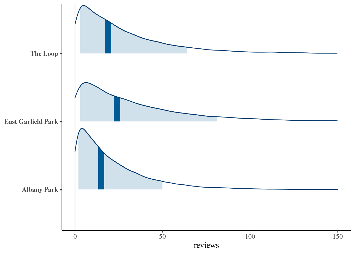
neighborhood = c("Albany Park", "East Garfield Park", "The Loop")))mcmc_areas(predicted_reviews, prob = 0.8) +
ggplot2::scale_y_discrete(
labels = c("Albany Park", "East Garfield Park", "The Loop")) +
xlim(0, 150) +
xlab("reviews")## Scale for y is already present.
## Adding another scale for y, which will replace the existing scale.
## Scale for x is already present.
## Adding another scale for x, which will replace the existing scale.## Warning: Removed 3 rows containing missing values (`geom_segment()`).