12.5 Prior Distribution

Assuming these priors are independent.

\[\begin{array}{rcl} Y_{i} | \beta_{0}, \beta_{1}, \beta_{2}, \beta_{3}, \sigma & \sim & \text{Pois}(\lambda_{i}) \\ \beta_{0c} & \sim & \text{N}(2, 0.5^{2}) \\ \beta_{1} & \sim & \text{N}(0, 0.17^{2}) \\ \beta_{2} & \sim & \text{N}(0, 4.97^{2}) \\ \beta_{3} & \sim & \text{N}(0, 5.60^{2}) \\ \end{array}\]

• “typical state” \(\lambda = 7\)

\[\log(\lambda) = \log(7) \approx 1.95 \approx 2\]

• logged number of laws \((2 \pm 2 \times 0.5)\)

\[(e^{1}, e^{3}) \approx (3, 20)\]

prior_summary(equality_model_prior)

## Priors for model 'equality_model_prior' 
## ------
## Intercept (after predictors centered)
##  ~ normal(location = 2, scale = 0.5)
## 
## Coefficients
##   Specified prior:
##     ~ normal(location = [0,0,0], scale = [2.5,2.5,2.5])
##   Adjusted prior:
##     ~ normal(location = [0,0,0], scale = [0.17,4.97,5.60])
## ------
## See help('prior_summary.stanreg') for more details

12.5.1 So Far

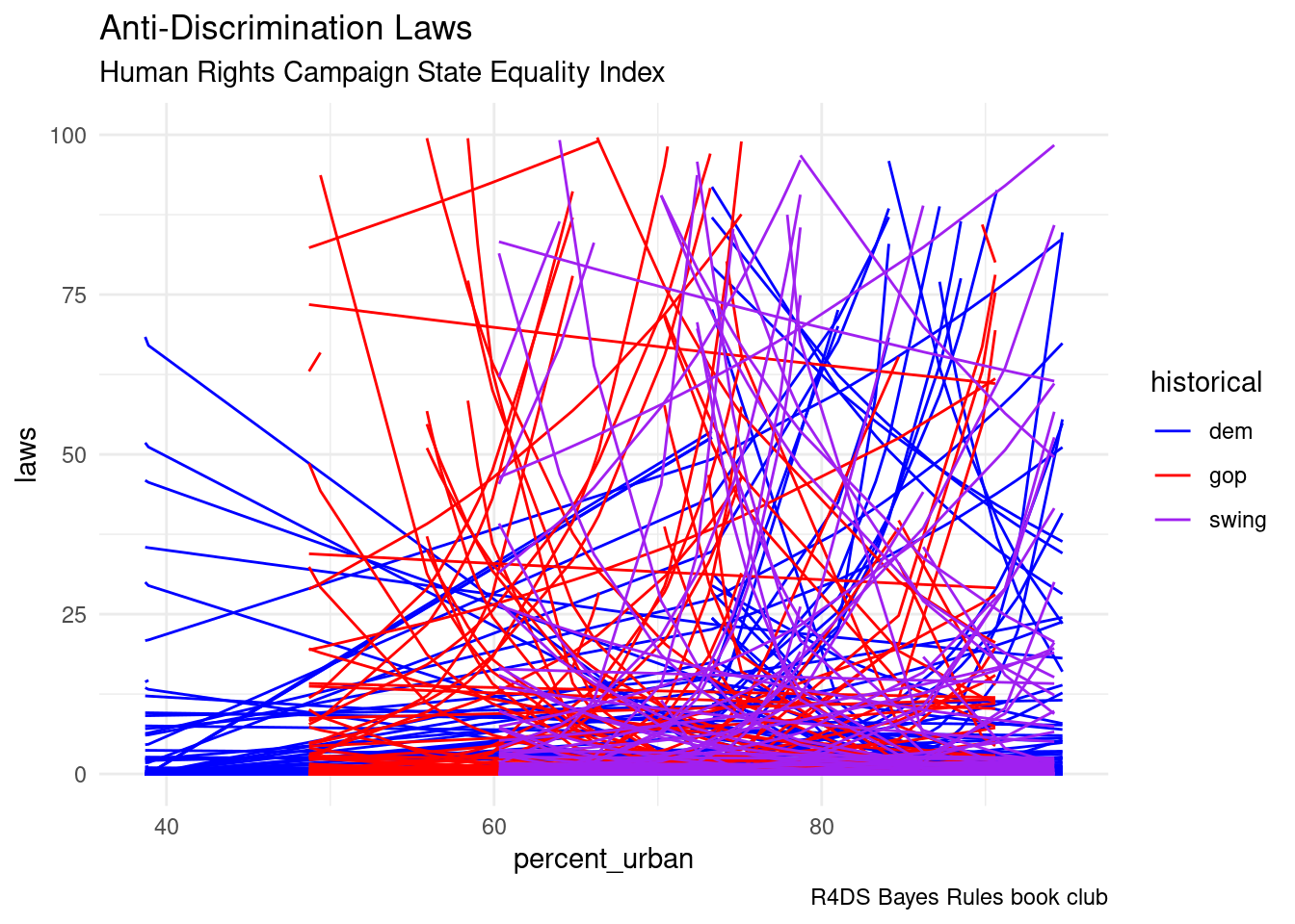
equality %>% 
  add_fitted_draws(equality_model_prior, n = 100) %>%
  ggplot(aes(x = percent_urban, y = laws, color = historical)) +
    geom_line(aes(y = .value, group = paste(historical, .draw))) +
  labs(title = "Anti-Discrimination Laws",
       subtitle = "Human Rights Campaign State Equality Index",
       caption = "R4DS Bayes Rules book club") +
  scale_color_manual(values = c("blue", "red", "purple")) +
  theme_minimal() + 
    ylim(0, 100)