11.7 Evaluating predictive accuracy using ELPD

# Calculate ELPD for the 4 models
set.seed(84735)
loo_1 <- loo(weather_model_1)
loo_2 <- loo(weather_model_2)
loo_3 <- loo(weather_model_3)
loo_4 <- loo(weather_model_4)

## Warning: Found 1 observation(s) with a pareto_k > 0.7. We recommend calling 'loo' again with argument 'k_threshold = 0.7' in order to calculate the ELPD without the assumption that these observations are negligible. This will refit the model 1 times to compute the ELPDs for the problematic observations directly.

# Results
c(loo_1$estimates[1], loo_2$estimates[1], 
  loo_3$estimates[1], loo_4$estimates[1])

## [1] -568.4233 -625.7383 -461.0916 -457.6155

# Compare the ELPD for the 4 models
loo_compare(loo_1, loo_2, loo_3, loo_4)

##                 elpd_diff se_diff
## weather_model_4    0.0       0.0 
## weather_model_3   -3.5       4.0 
## weather_model_1 -110.8      18.1 
## weather_model_2 -168.1      21.5

11.7.1 The bias-variance trade-off

Explore the bias-variance trade-off speaks to the performance of a model across multiple datasets:

first simulate the posteriors for each model
calculate raw and cross-validated posterior prediction summaries for each model

# Take 2 separate samples
set.seed(84735)
weather_shuffle <- weather_australia %>% 
  filter(temp3pm < 30, 
         location == "Wollongong") %>% 
  sample_n(nrow(.))
sample_1 <- weather_shuffle %>% head(40)
sample_2 <- weather_shuffle %>% tail(40)

g <- ggplot(sample_1, aes(y = temp3pm, 
                          x = day_of_year)) + 
  geom_point()


g + geom_smooth(method = "lm", se = FALSE)

## `geom_smooth()` using formula = 'y ~ x'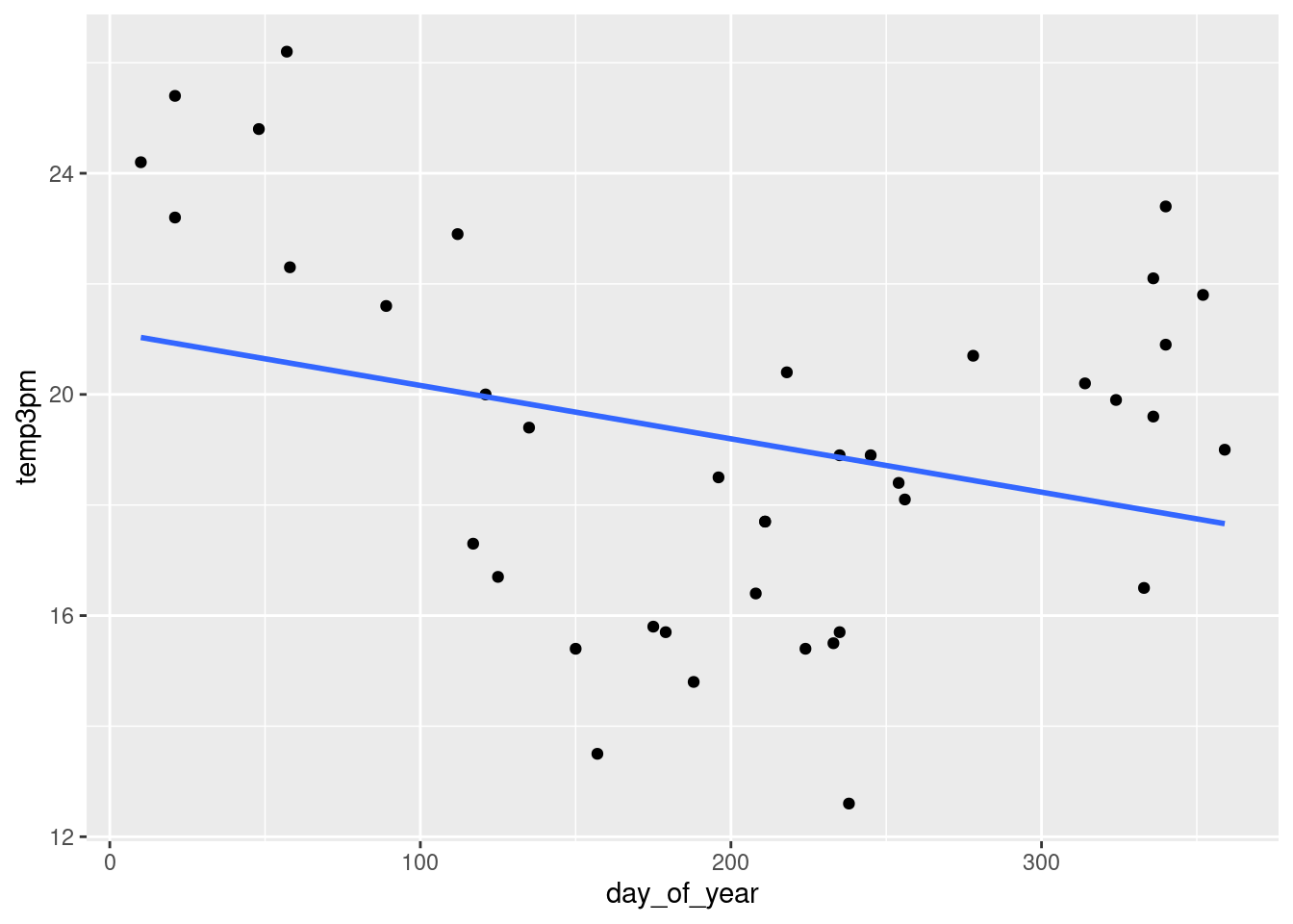

g + stat_smooth(method = "lm", 
                se = FALSE, 
                formula = y ~ poly(x, 2))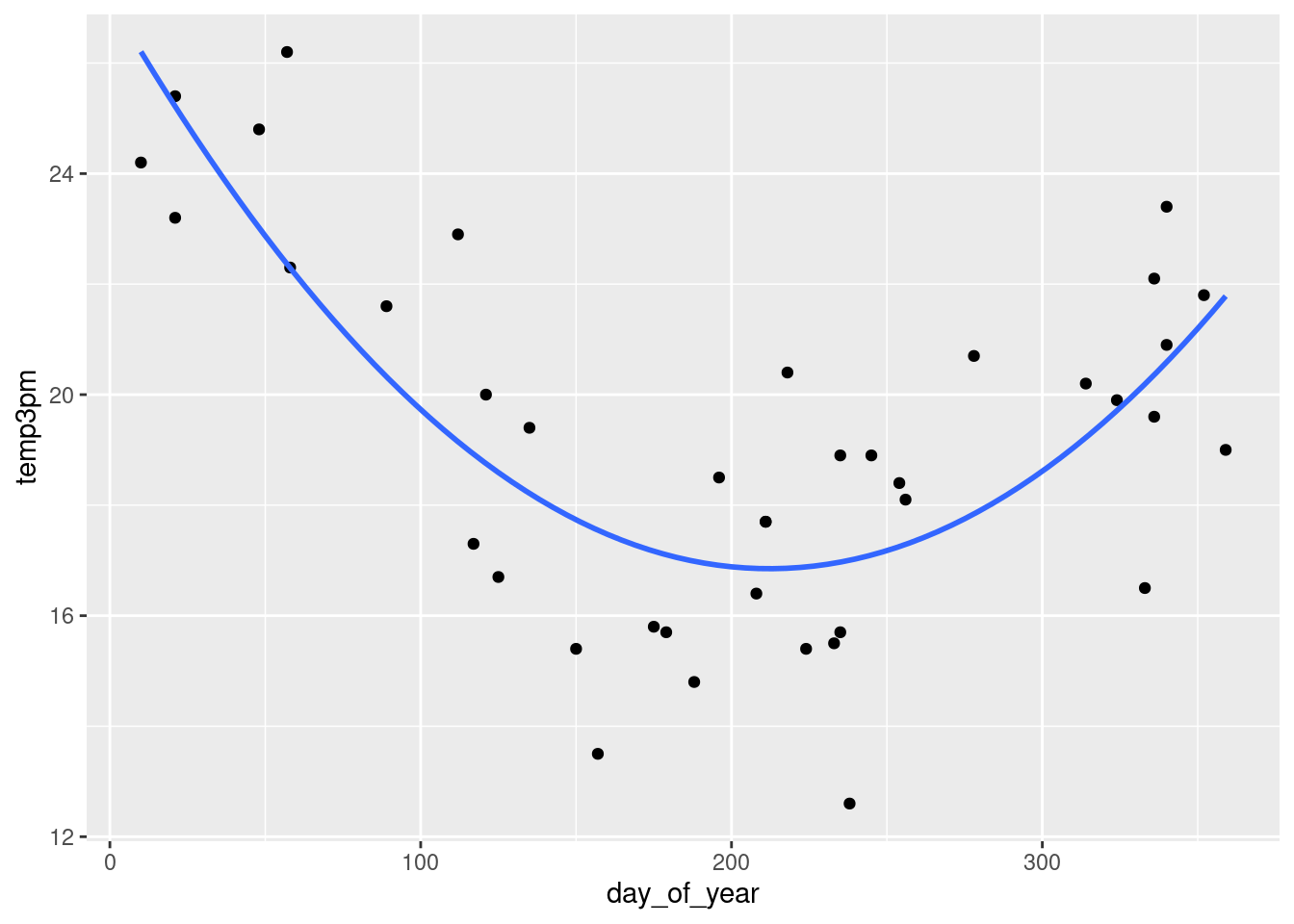

g + stat_smooth(method = "lm", 
                se = FALSE, 
                formula = y ~ poly(x, 12))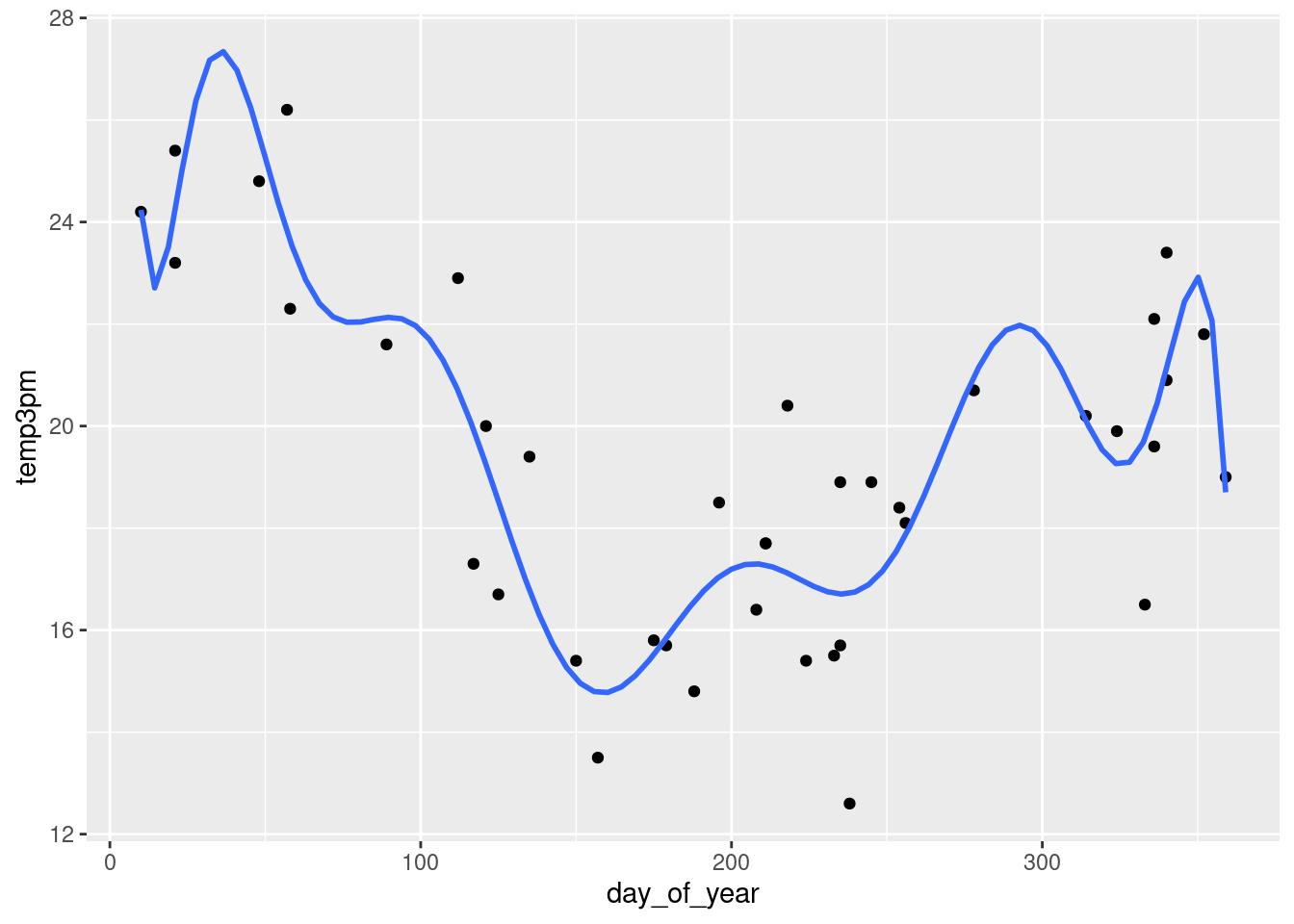

model_1 <- stan_glm(
  temp3pm ~ day_of_year,
  data = sample_1, family = gaussian,
  prior_intercept = normal(25, 5),
  prior = normal(0, 2.5, autoscale = TRUE),
  prior_aux = exponential(1, autoscale = TRUE),
  chains = 4, iter = 5000*2, seed = 84735)

# Ditto the syntax for models 2 and 3
model_2 <- stan_glm(temp3pm ~ poly(day_of_year, 2),
                    data = sample_1, 
                    family = gaussian,
                    prior_intercept = normal(25, 5),
                    prior = normal(0, 2.5, 
                                   autoscale = TRUE),
                    prior_aux = exponential(1, autoscale = TRUE),
                    chains = 4, 
                    iter = 5000*2, 
                    seed = 84736)
model_3 <- stan_glm(temp3pm ~ poly(day_of_year, 12),
                    data = sample_1, 
                    family = gaussian,
                    prior_intercept = normal(25, 5),
                    prior = normal(0, 2.5, 
                                   autoscale = TRUE),
                    prior_aux = exponential(1, autoscale = TRUE),
                    chains = 4, 
                    iter = 5000*2, 
                    seed = 84737)

set.seed(84735)
prediction_summary(model = model_1, data = sample_1)

##        mae mae_scaled within_50 within_95
## 1 2.788129   0.819851     0.475         1

prediction_summary_cv(model = model_1, 
                      data = sample_1, 
                      k = 10)$cv

##       mae mae_scaled within_50 within_95
## 1 2.82925  0.8308622     0.475     0.975