16.3 No pooled model
ggplot(spotify, aes(x = popularity, group = artist)) +
  geom_density()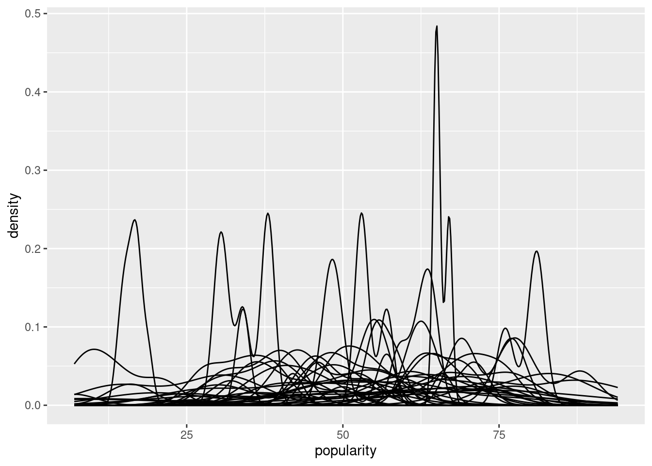
Key points:
popularity can differ from one artist to an other
some artist have a “stable” popularity across their song and some not
Let change our model to reflect that:
\[Y_{ij}|\mu_j, \sigma \sim N(\mu_{j}, \sigma^2 ) \] \(\mu_{j}\) : mean song popularity for artist \(j\)
\(\sigma\) : standard deviation in popularity from song to song within each artist
spotify_no_pooled <- stan_glm(
  popularity ~ artist - 1,
  data = spotify, family = gaussian,
  prior = normal(50, 2.5, autoscale = TRUE),
  prior_aux = exponential(1, autoscale = TRUE),
  chains = 4, iter = 5000*2, seed = 84735)
16.3.1 Same Quiz but with no pooling!!
3 artist:
- Mia X, artist with the lowest mean popularity in our data set
- Beyoncé, artist with nearly the highest mean popularity in our data set
- Mohsen Beats, an artist not in out data set
set.seed(84735)
predictions_no <- posterior_predict(
spotify_no_pooled, newdata = artist_means)
# Plot the posterior predictive intervals
ppc_intervals(artist_means$popularity, yrep = predictions_no,
prob_outer = 0.80) +
ggplot2::scale_x_continuous(labels = artist_means$artist,
breaks = 1:nrow(artist_means)) +
xaxis_text(angle = 90, hjust = 1)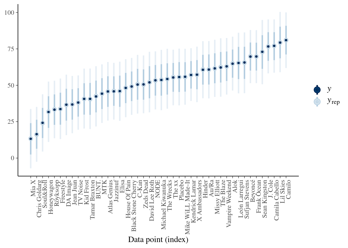 Two drawbacks:
Ignoring other artist when modeling for one specific artist (what happens when fewer data point)
If we assume no other artists help us understanding popularity of a specific artist we can not generalize to artist outside of our data set.