17.2 Hierarchical Model with varying intercept

17.2.1 Model buildings

17.2.1.1 Layer 1 Within-group: within runner

\[Y_{ij} | \beta_0, \beta_1, \sigma_j \sim N(\mu_{ij}, \sigma_j^2)\]

We added a bunch of \(j\)! So now we have runner specific mean (\(\mu_{ij}\)) and the variance with a runner (\(\sigma_j\))

\[\mu_{ij} = \beta_{0j} + \beta_1X_{ij}\] Here we are using a specific intercept for each runner (\(\beta_{oj}\)) but we are still using a global age coefficient (\(\beta_1\)).

17.2.1.2 Layer 2: Between Runners

Quizz!

Which of our current parameters (\(\beta_{0j}, \beta_1, \sigma_y\)) do we need to model in the next layer? (hint:title)

\[\beta_{0j} | \beta_{0}, \sigma_0 \overset{\text{ind}}{\sim} N(\beta_0, \sigma_0^2)\]

\(\beta_{0j}\) is our intercept for each runner and it follow a normal distribution with the global average of intercept (\(\beta_0\)) and the between-group variability (\(\sigma_0\)).

Now quiz!

For Which model parameters must we specify priors in the final layer of our hierarchical regression model?

\[\beta_{0c} \sim N(m_0, s_0^2)\]

\[\beta_1 \sim N(m_1, s_1^2)\]

\[\sigma_y \sim Exp(l_y)\]

\[\sigma_0 \sim Exp(l_0)\]

Normal hierarchical regression assumptions:

• structure of the data: conditioned on \(X_{ij}\), \(Y_{ij}\) on any group j is independant of other group k but different data point within the same group are correlated

• structure of the relationship: Linear relation

• structure of variability within groups: Within any group j at any predictor value \(X_{ij}\) the observed values of \(Y_{ij}\) will vary normally

• Structure of variability between groups

17.2.1.3 Tuning the prior

\[\beta_{0c} \sim N(100, 10^2)\] runing tine is around 80 - 120 mins

\[\beta_1 \sim N(2.5, 1^2)\] We just know that it increase and it can range from 0.5 to 4.5 mins / year (on average)

\[\sigma_y \sim Exp(0.078)\]

\[\sigma_0 \sim Exp(1)\]

Then we use weakly informative priors.

running_model_1_prior <- stan_glmer(
  net ~ age + (1 | runner),  # formula
  data = running, family = gaussian,
  prior_intercept = normal(100, 10),
  prior = normal(2.5, 1), 
  prior_aux = exponential(1, autoscale = TRUE),
  prior_covariance = decov(reg = 1, conc = 1, shape = 1, scale = 1),
  chains = 4, iter = 5000*2, seed = 84735, 
  prior_PD = TRUE) # just the prior

## 
## SAMPLING FOR MODEL 'continuous' NOW (CHAIN 1).
## Chain 1: 
## Chain 1: Gradient evaluation took 2.2e-05 seconds
## Chain 1: 1000 transitions using 10 leapfrog steps per transition would take 0.22 seconds.
## Chain 1: Adjust your expectations accordingly!
## Chain 1: 
## Chain 1: 
## Chain 1: Iteration:    1 / 10000 [  0%]  (Warmup)
## Chain 1: Iteration: 1000 / 10000 [ 10%]  (Warmup)
## Chain 1: Iteration: 2000 / 10000 [ 20%]  (Warmup)
## Chain 1: Iteration: 3000 / 10000 [ 30%]  (Warmup)
## Chain 1: Iteration: 4000 / 10000 [ 40%]  (Warmup)
## Chain 1: Iteration: 5000 / 10000 [ 50%]  (Warmup)
## Chain 1: Iteration: 5001 / 10000 [ 50%]  (Sampling)
## Chain 1: Iteration: 6000 / 10000 [ 60%]  (Sampling)
## Chain 1: Iteration: 7000 / 10000 [ 70%]  (Sampling)
## Chain 1: Iteration: 8000 / 10000 [ 80%]  (Sampling)
## Chain 1: Iteration: 9000 / 10000 [ 90%]  (Sampling)
## Chain 1: Iteration: 10000 / 10000 [100%]  (Sampling)
## Chain 1: 
## Chain 1:  Elapsed Time: 0.568 seconds (Warm-up)
## Chain 1:                0.588 seconds (Sampling)
## Chain 1:                1.156 seconds (Total)
## Chain 1: 
## 
## SAMPLING FOR MODEL 'continuous' NOW (CHAIN 2).
## Chain 2: 
## Chain 2: Gradient evaluation took 1.6e-05 seconds
## Chain 2: 1000 transitions using 10 leapfrog steps per transition would take 0.16 seconds.
## Chain 2: Adjust your expectations accordingly!
## Chain 2: 
## Chain 2: 
## Chain 2: Iteration:    1 / 10000 [  0%]  (Warmup)
## Chain 2: Iteration: 1000 / 10000 [ 10%]  (Warmup)
## Chain 2: Iteration: 2000 / 10000 [ 20%]  (Warmup)
## Chain 2: Iteration: 3000 / 10000 [ 30%]  (Warmup)
## Chain 2: Iteration: 4000 / 10000 [ 40%]  (Warmup)
## Chain 2: Iteration: 5000 / 10000 [ 50%]  (Warmup)
## Chain 2: Iteration: 5001 / 10000 [ 50%]  (Sampling)
## Chain 2: Iteration: 6000 / 10000 [ 60%]  (Sampling)
## Chain 2: Iteration: 7000 / 10000 [ 70%]  (Sampling)
## Chain 2: Iteration: 8000 / 10000 [ 80%]  (Sampling)
## Chain 2: Iteration: 9000 / 10000 [ 90%]  (Sampling)
## Chain 2: Iteration: 10000 / 10000 [100%]  (Sampling)
## Chain 2: 
## Chain 2:  Elapsed Time: 0.562 seconds (Warm-up)
## Chain 2:                0.593 seconds (Sampling)
## Chain 2:                1.155 seconds (Total)
## Chain 2: 
## 
## SAMPLING FOR MODEL 'continuous' NOW (CHAIN 3).
## Chain 3: 
## Chain 3: Gradient evaluation took 1.5e-05 seconds
## Chain 3: 1000 transitions using 10 leapfrog steps per transition would take 0.15 seconds.
## Chain 3: Adjust your expectations accordingly!
## Chain 3: 
## Chain 3: 
## Chain 3: Iteration:    1 / 10000 [  0%]  (Warmup)
## Chain 3: Iteration: 1000 / 10000 [ 10%]  (Warmup)
## Chain 3: Iteration: 2000 / 10000 [ 20%]  (Warmup)
## Chain 3: Iteration: 3000 / 10000 [ 30%]  (Warmup)
## Chain 3: Iteration: 4000 / 10000 [ 40%]  (Warmup)
## Chain 3: Iteration: 5000 / 10000 [ 50%]  (Warmup)
## Chain 3: Iteration: 5001 / 10000 [ 50%]  (Sampling)
## Chain 3: Iteration: 6000 / 10000 [ 60%]  (Sampling)
## Chain 3: Iteration: 7000 / 10000 [ 70%]  (Sampling)
## Chain 3: Iteration: 8000 / 10000 [ 80%]  (Sampling)
## Chain 3: Iteration: 9000 / 10000 [ 90%]  (Sampling)
## Chain 3: Iteration: 10000 / 10000 [100%]  (Sampling)
## Chain 3: 
## Chain 3:  Elapsed Time: 0.571 seconds (Warm-up)
## Chain 3:                0.594 seconds (Sampling)
## Chain 3:                1.165 seconds (Total)
## Chain 3: 
## 
## SAMPLING FOR MODEL 'continuous' NOW (CHAIN 4).
## Chain 4: 
## Chain 4: Gradient evaluation took 1.5e-05 seconds
## Chain 4: 1000 transitions using 10 leapfrog steps per transition would take 0.15 seconds.
## Chain 4: Adjust your expectations accordingly!
## Chain 4: 
## Chain 4: 
## Chain 4: Iteration:    1 / 10000 [  0%]  (Warmup)
## Chain 4: Iteration: 1000 / 10000 [ 10%]  (Warmup)
## Chain 4: Iteration: 2000 / 10000 [ 20%]  (Warmup)
## Chain 4: Iteration: 3000 / 10000 [ 30%]  (Warmup)
## Chain 4: Iteration: 4000 / 10000 [ 40%]  (Warmup)
## Chain 4: Iteration: 5000 / 10000 [ 50%]  (Warmup)
## Chain 4: Iteration: 5001 / 10000 [ 50%]  (Sampling)
## Chain 4: Iteration: 6000 / 10000 [ 60%]  (Sampling)
## Chain 4: Iteration: 7000 / 10000 [ 70%]  (Sampling)
## Chain 4: Iteration: 8000 / 10000 [ 80%]  (Sampling)
## Chain 4: Iteration: 9000 / 10000 [ 90%]  (Sampling)
## Chain 4: Iteration: 10000 / 10000 [100%]  (Sampling)
## Chain 4: 
## Chain 4:  Elapsed Time: 0.564 seconds (Warm-up)
## Chain 4:                0.589 seconds (Sampling)
## Chain 4:                1.153 seconds (Total)
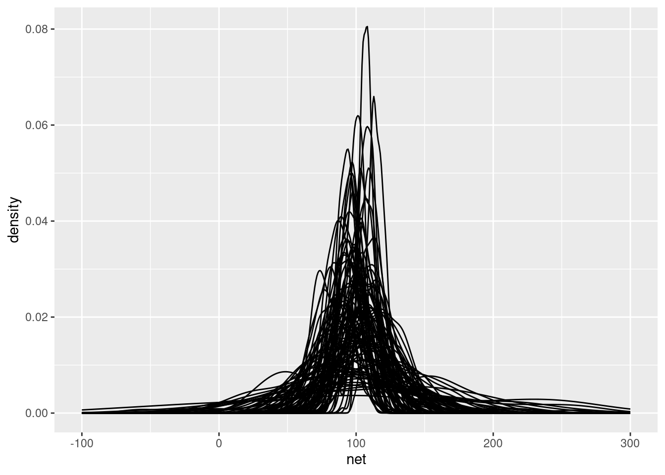
## Chain 4:

running |>
  # here we just used 100 sims
  add_predicted_draws(running_model_1_prior, n = 100) |>
  ggplot(aes(x = net)) +
    geom_density(aes(x = .prediction, group = .draw)) +
    xlim(-100,300)

## Warning: 
## In add_predicted_draws(): The `n` argument is a deprecated alias for `ndraws`.
## Use the `ndraws` argument instead.
## See help("tidybayes-deprecated").

## Warning: Removed 46 rows containing non-finite values (`stat_density()`).