17.6 Posterior prediction

We will use running_model_1.

We will try to predict for runner1, runner10 and Miles (one of the authors) when they will be 61 years old.

running |> 
  filter(runner %in% c("1", "10")) |> 
  ggplot(data = _ , aes(x = age, y = net)) + 
    geom_point() + 
    facet_grid(~ runner) + 
    lims(x = c(54, 61))

## Warning: Removed 1 rows containing missing values (`geom_point()`).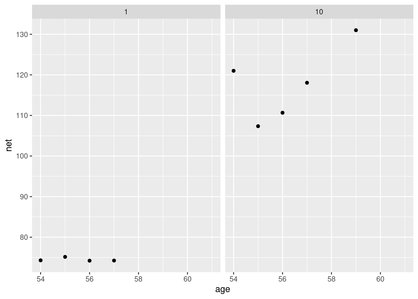

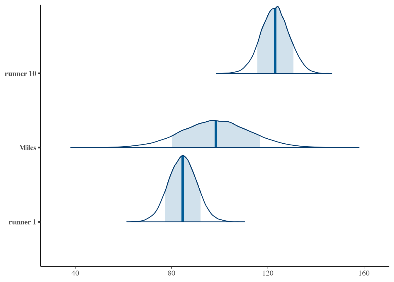
We will have two sources of uncertainty in runner 1 and 10 (within-group sampling variability \(\sigma_y\), posterior variability, \(\beta_{0j}\), \(\beta_1\) and \(\sigma_y\)) and for Miles we need to add the between-group sampling variability (\(\sigma_0\)).

set.seed(84735)
predict_next_race <- posterior_predict(
  running_model_1, 
  newdata = data.frame(runner = c("1", "Miles", "10"),
                       age = c(61, 61, 61)))

apply(predict_next_race, 2, median)

##         1         2         3 
##  84.63351  98.34833 123.02690

mcmc_areas(predict_next_race, prob = 0.8) +
 ggplot2::scale_y_discrete(labels = c("runner 1", "Miles", "runner 10"))

## Scale for y is already present.
## Adding another scale for y, which will replace the existing scale.