13.2 Simulating the posterior

ggplot(weather, aes(x = humidity9am, y = raintomorrow)) + 
  geom_jitter(size = 0.2)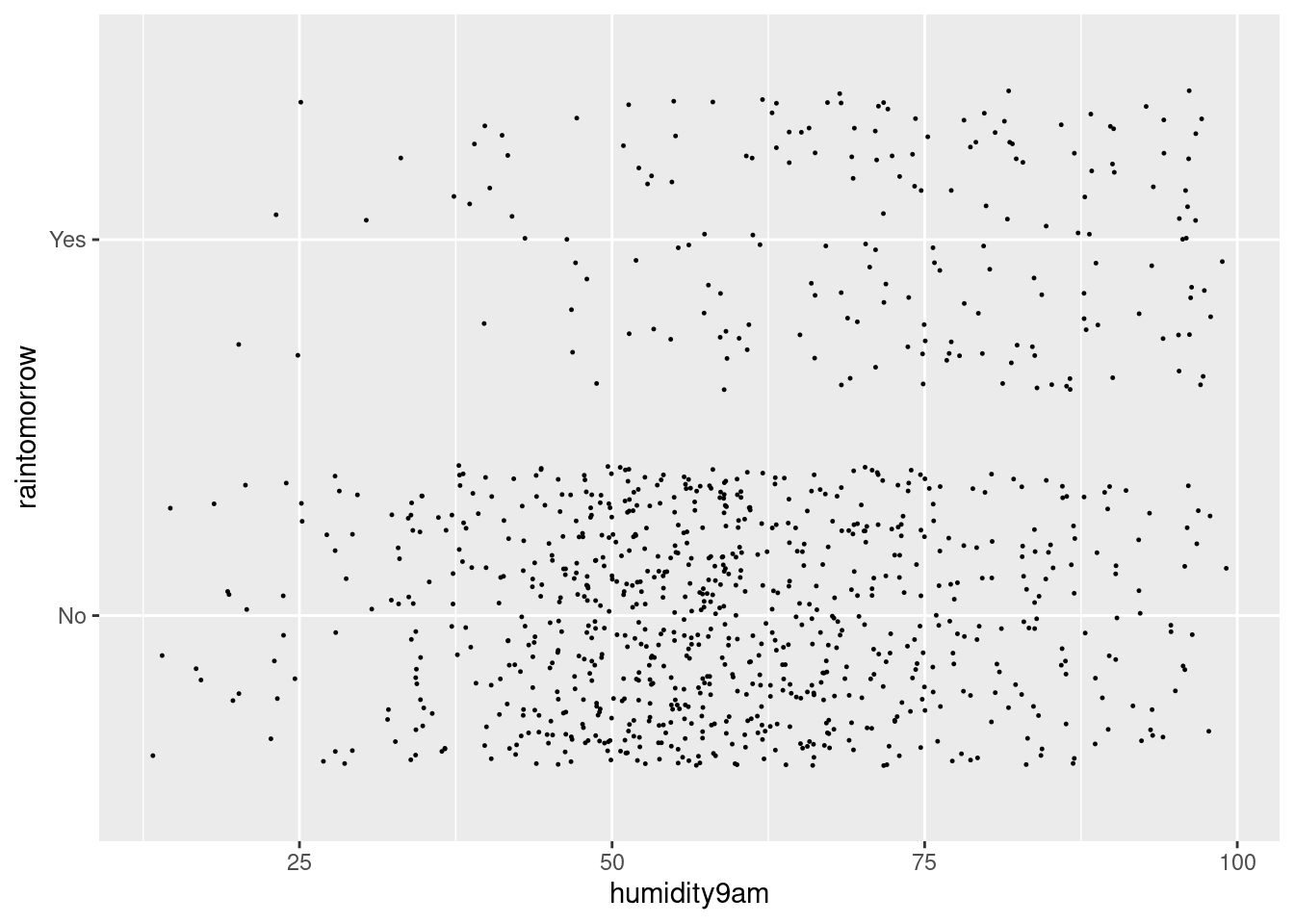

Calculate & plot the rain rate by humidity bracket:

weather %>% 
  mutate(humidity_bracket = 
           cut(humidity9am, 
               breaks = seq(10, 100, by = 10))) %>% 
  group_by(humidity_bracket) %>% 
  summarize(rain_rate = mean(raintomorrow == "Yes")) %>% 
  ggplot(aes(x = humidity_bracket, y = rain_rate)) + 
    geom_point() + 
    theme(axis.text.x = element_text(angle = 45, vjust = 0.5))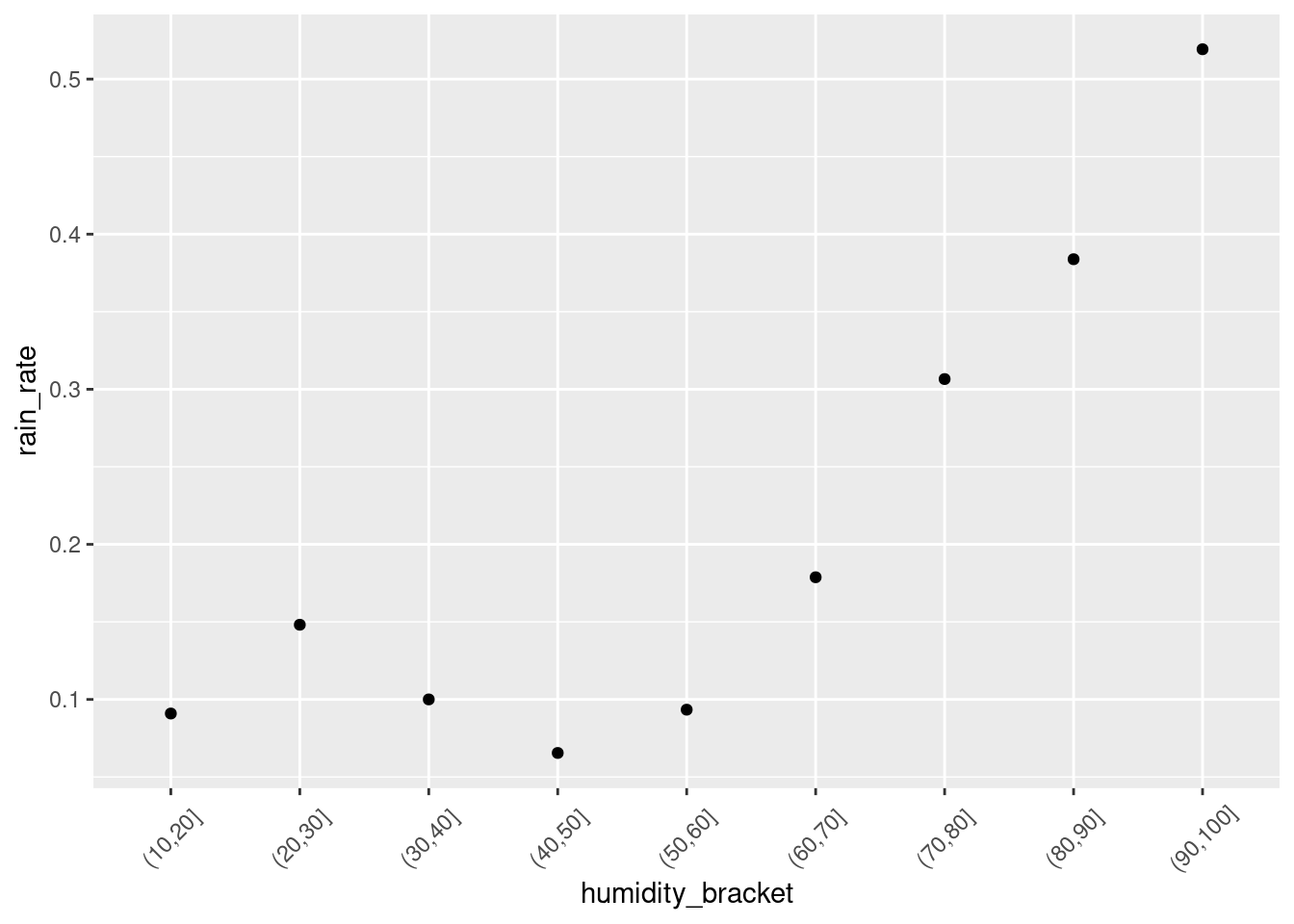

Simulate the model:

prior_PD = FALSE

rain_model_1 <- update(rain_model_prior, prior_PD = FALSE)
rain_model_1

Check the stability of the simulation results before proceeding:

MCMC trace, density, & autocorrelation plots

mcmc_trace(rain_model_1)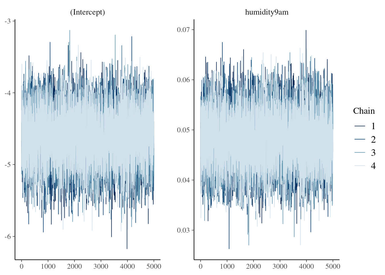

mcmc_dens_overlay(rain_model_1)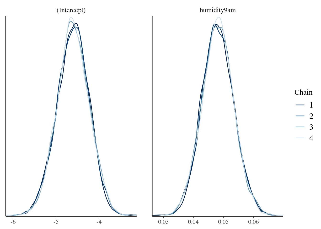

mcmc_acf(rain_model_1)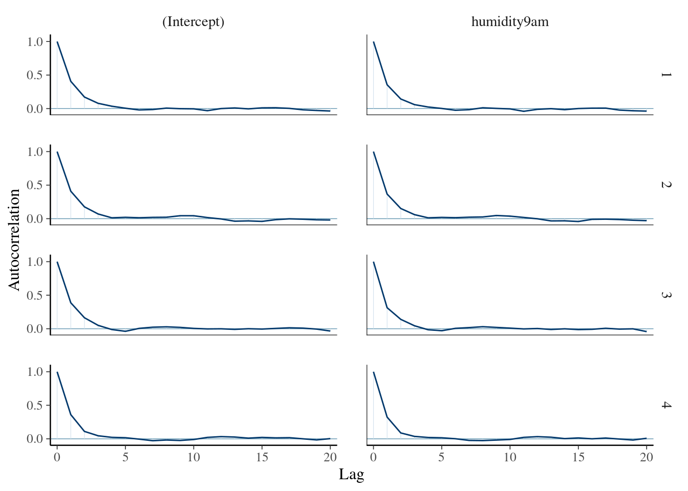

Plot the posterior model results:

weather %>%
  add_fitted_draws(rain_model_1, n = 100) %>%
  ggplot(aes(x = humidity9am, y = raintomorrow)) +
    geom_line(aes(y = .value, group = .draw), alpha = 0.15) + 
    labs(y = "probability of rain")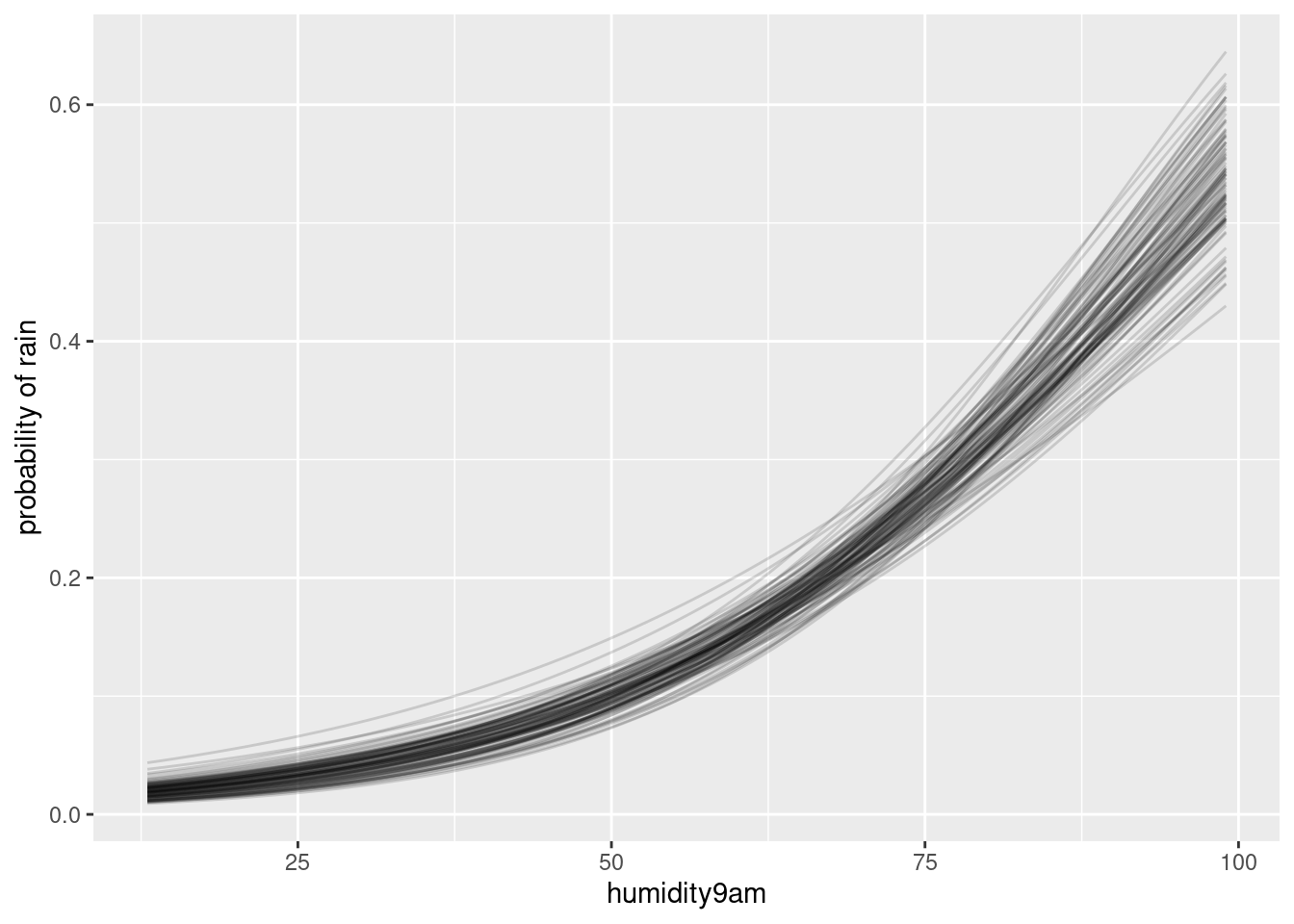

Posterior summaries on the log(odds) scale

posterior_interval(rain_model_1, prob = 0.80)

##                     10%         90%
## (Intercept) -5.08784667 -4.13449813
## humidity9am  0.04146719  0.05487265

Posterior summaries on the odds scale

exp(posterior_interval(rain_model_1, prob = 0.80))

##                     10%       90%
## (Intercept) 0.006171294 0.0160107
## humidity9am 1.042338958 1.0564061