10.7 How Accurate are the Posterior Predictive Models?

Here we explore three approaches to evaluating predictive quality

10.7.1 Posterior predictive summaries

• median absolute error (MAE)

• scaled median absolute error (AKA relative error)

• within_50 and within_95

  • proportion of data within those posterior prediction intervals

set.seed(84735)
prediction_summary(bike_model, data = bikes)

##        mae mae_scaled within_50 within_95
## 1 990.0297  0.7709971     0.438     0.968

set.seed(84735)
predict_75 <- bike_model_df %>% 
  mutate(mu = `(Intercept)` + temp_feel*75,
         y_new = rnorm(20000, mean = mu, sd = sigma))

# Plot the posterior predictive model
ggplot(predict_75, aes(x = y_new)) + 
  geom_density()+
  geom_vline(aes(xintercept = 6228))+
  labs(title="The posterior predictive model of ridership on October 22, 2012,\na 75-degree day. The actual Y = 6228 riders observed that day are\nmarked by the vertical line.")+
  ggthemes::theme_fivethirtyeight()+
  theme(plot.title = element_text(size=10))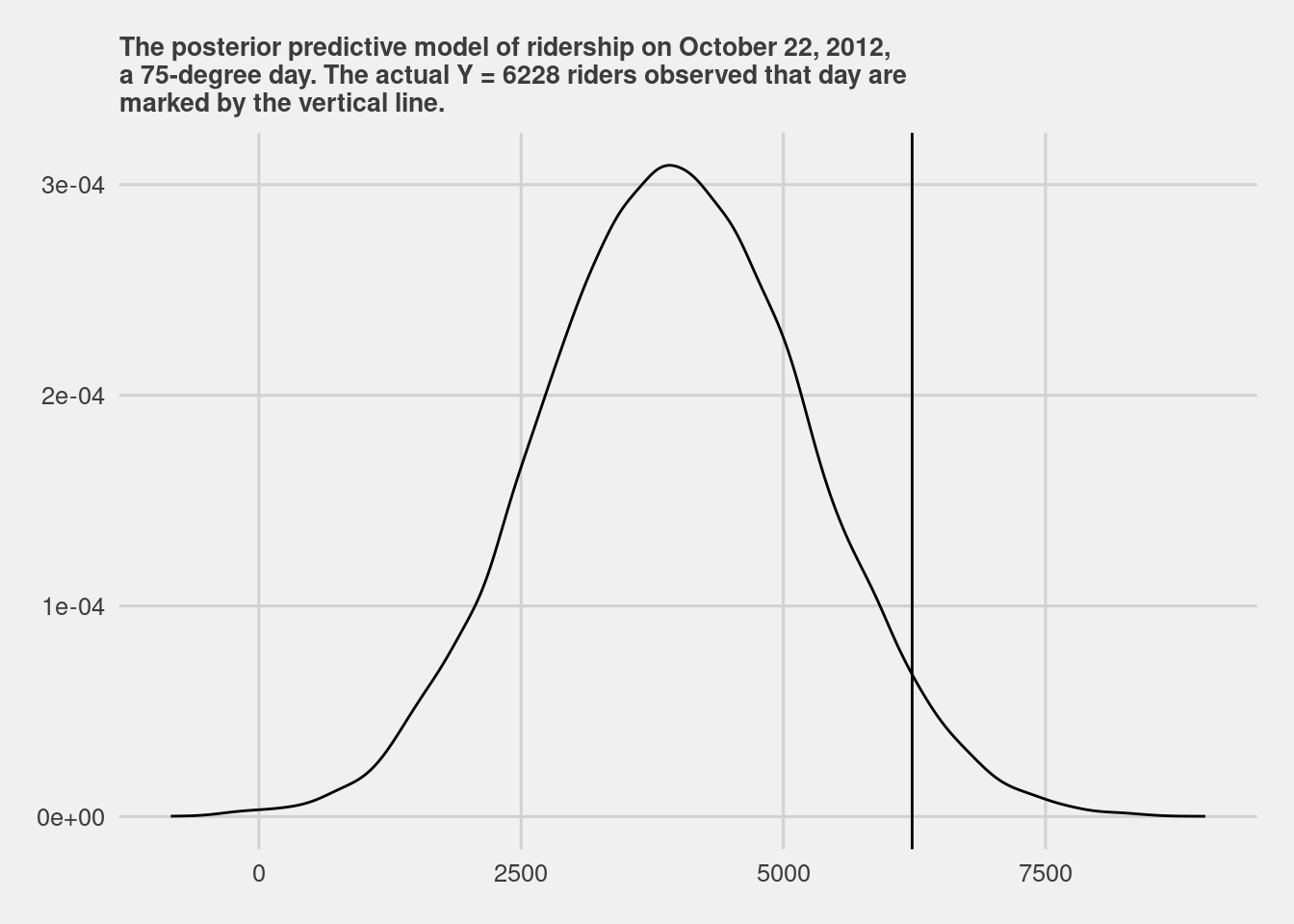

set.seed(84735)
predictions <- posterior_predict(bike_model, newdata = bikes)
dim(predictions)

## [1] 20000   500

ppc_intervals(bikes$rides, yrep = predictions, x = bikes$temp_feel, 
              prob = 0.5, prob_outer = 0.95)+
  labs(title="Posterior Predictive Medians",
       subtitle = "with prediction intervals",
       caption = "R4DS Book Club",
       x = "temperature feel",
       y = "ridership")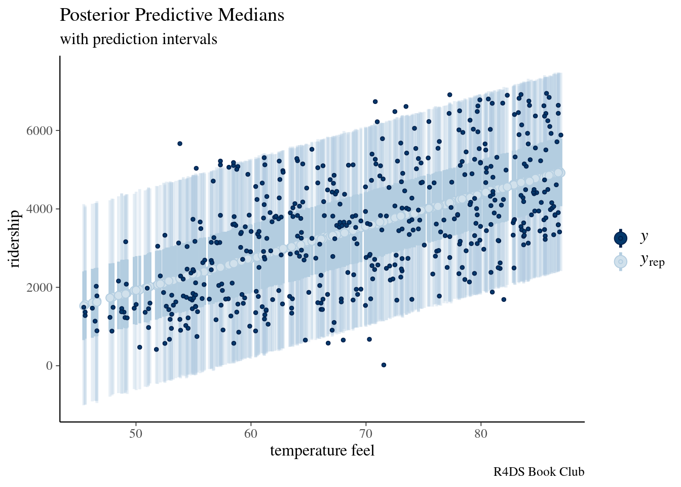

The posterior predictive medians (light blue dots), 50% prediction intervals (wide, short blue bars),and 95% prediction intervals (narrow, long blue bars) for each day in the bikes data set, along with the corresponding observed data points (dark blue dots).

10.7.2 Cross-validation

To see how well our model generalizes to new data beyond our original sample, we can estimate these properties using cross-validation techniques.

• Train the model
• Test the model

set.seed(84735)
cv_procedure <- prediction_summary_cv(model = bike_model, 
                                      data = bikes, 
                                      k = 10)

cv_procedure$folds %>% head

##   fold       mae mae_scaled within_50 within_95
## 1    1  990.1664  0.7700186      0.46      0.98
## 2    2  965.4630  0.7432483      0.42      1.00
## 3    3  951.2222  0.7303042      0.42      0.98
## 4    4 1018.4456  0.7906957      0.46      0.98
## 5    5 1161.7817  0.9091292      0.36      0.96
## 6    6  936.9525  0.7322033      0.46      0.94

cv_procedure$cv

##        mae mae_scaled within_50 within_95
## 1 1029.254  0.8015919     0.422     0.968

10.7.3 Expected log-predictive density

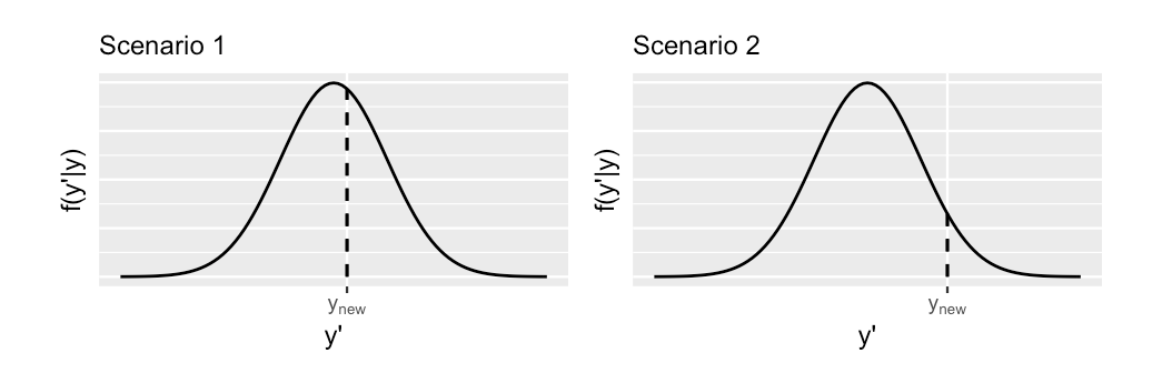
(#fig:10.21)Two hypothetical posterior predictive pdfs for Y new, the yet unobserved ridership on a new day. The eventual observed value of y new, is represented by a dashed vertical line

ELPD measures the average log posterior predictive pdf, across all possible new data points. The higher the ELPD, the better. Higher ELPDs indicate greater posterior predictive accuracy when using our model to predict new data points.

The loo() function in the {rstanarm} package utilizes leave-one-out cross-validation to estimate the ELPD of a given model:

model_elpd <- loo(bike_model)
model_elpd$estimates

##              Estimate         SE
## elpd_loo -4289.034580 13.1127988
## p_loo        2.503113  0.1648177
## looic     8578.069161 26.2255976

These estimates are very context dependent, but are more useful when comparing models.