5.14 Normal Model

$$Y \sim N(\mu,\sigma^2)$$

$$f(y)=\frac{1}{\sqrt{2 \pi \sigma^2}}exp\begin{bmatrix} -\frac{(y-\mu)^2}{2\sigma^2/n}\end{bmatrix}$$ for $y \epsilon (-\infty,\infty)$

  plot_normal(mean,sd)

library(bayesrules)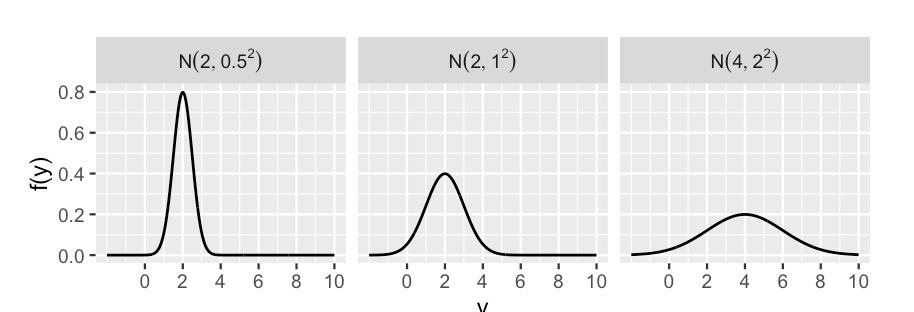

5.14.1 Prior X Likelihood = Posterior

$f(\vec{y}|\mu)$ x $L(\mu|\vec{y})$

Starting from the prior model:

$$\mu \sim N(6.5,0.4^2)$$

We are considering the adults with experience of concussion, in the football dataset.

library(tidyverse)
football%>%head

##     group years volume
## 1 control     0  6.175
## 2 control     0  6.220
## 3 control     0  6.360
## 4 control     0  6.465
## 5 control     0  6.540
## 6 control     0  6.780

football%>%count(group)

##           group  n
## 1       control 25
## 2    fb_concuss 25
## 3 fb_no_concuss 25

Let’s see the mean:

football%>%
  filter(group == "fb_concuss")%>%
  summarise(mean=mean(volume),sd=sd(volume))

##     mean        sd
## 1 5.7346 0.5933976

concussion_subjects <- football%>%
  filter(group == "fb_concuss")

concussion_subjects%>%
  ggplot(aes(x = volume)) + 
  geom_density()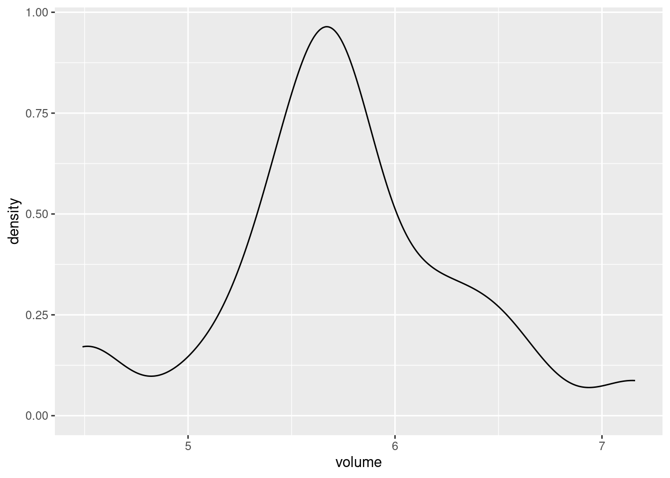

$$L(y|\vec{y}) \propto exp \begin{bmatrix} -\frac{(5.735-\mu)}{2(0.5^2/25)}\end{bmatrix}$$

plot_normal_likelihood(y = concussion_subjects$volume, sigma = 0.5)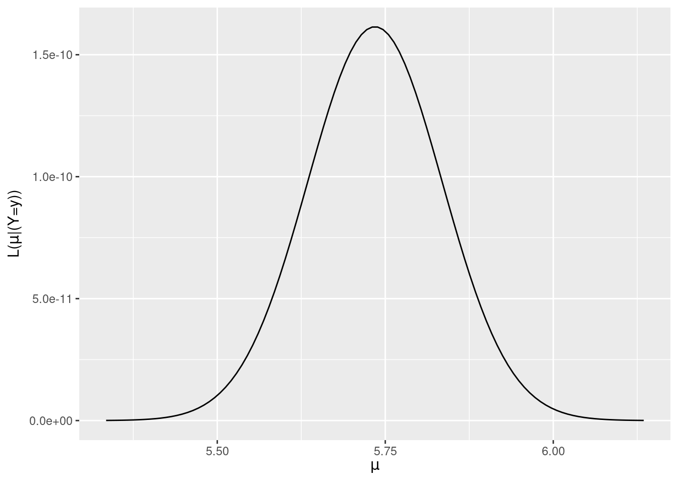

plot_normal_normal(mean = 6.5, sd = 0.4, sigma = 0.5,
                   y_bar = 5.735, n = 25)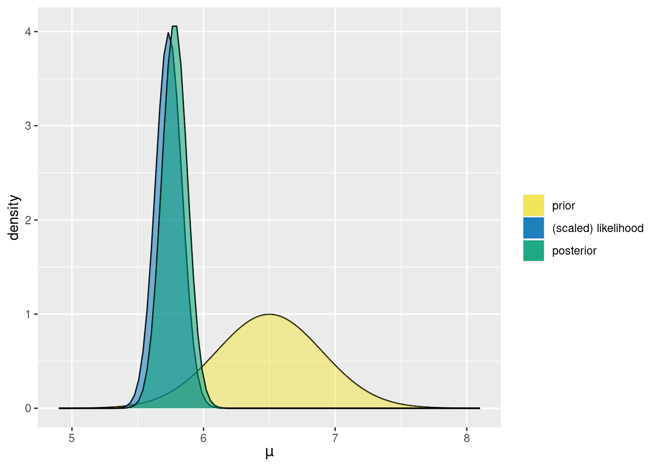

summarize_normal_normal(mean = 6.5, sd = 0.4, sigma = 0.5,
                        y_bar = 5.735, n = 25)

##       model mean mode         var         sd
## 1     prior 6.50 6.50 0.160000000 0.40000000
## 2 posterior 5.78 5.78 0.009411765 0.09701425