2.7 Building a Bayesian model for random variables

Here we will be modelling the probability (\(\pi\)) of Kasparov defeating Deep Blue in a game of chess.

2.7.1 Prior probability model

This is based on the matches played between Kasparov and Deep Blue in 1996.

\(\pi\)	0.2	0.5	0.8	Total
\(f(\pi)\)	10.0%	25.0%	65.0%	100.0%

R code for prior probability model:

pi <- c(0.2, 0.5, 0.8)
prior_prob <- c(0.1, 0.25, 0.65)

2.7.2 Data model

The number of matches won (\(Y\)) by Kasparov in the 1997 encounter will serve as the data in this setup.

In the end Kasparov just one out of the six matches played in 1997, i.e., \(Y = 1\)

R code for binomial data model (likelihood function):

likelihoods <- map_dbl(pi, ~dbinom(1, 6, .x))

ggplot(mapping = aes(x = pi, y = likelihoods)) +
  geom_point(size = 3) +
  geom_segment(aes(xend = pi, yend = 0)) +
  scale_x_continuous(breaks = pi) +
  xlab(TeX(r"($\pi$)")) +
  ylab(TeX(r"($L(\pi | y = 1)$)"))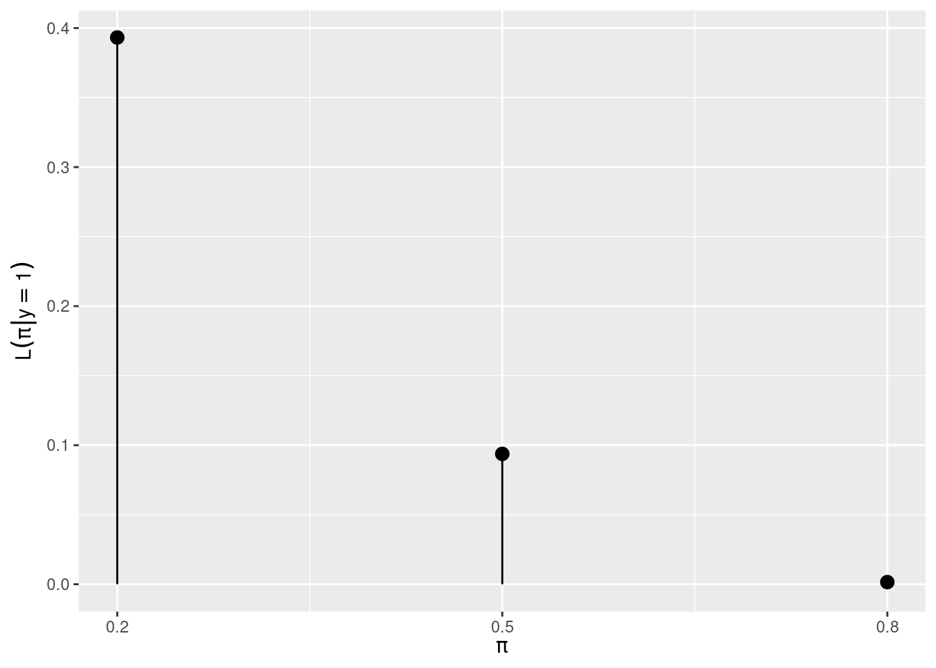

2.7.3 Posterior probability model

We can now combine the prior and likelihood to derive the posterior probabilities.

R code for posterior probability model:

posterior_prob <- prior_prob * likelihoods / sum(prior_prob * likelihoods)

tibble(pi = pi, prior = prior_prob, posterior = posterior_prob) |> 
  pivot_longer(cols = -pi, values_to = "probability") |> 
  mutate(name = fct_rev(name)) |> 
  ggplot() +
  geom_col(aes(pi, probability, fill = name), position = "dodge") +
  scale_x_continuous(breaks = pi) +
  theme(legend.title = element_blank())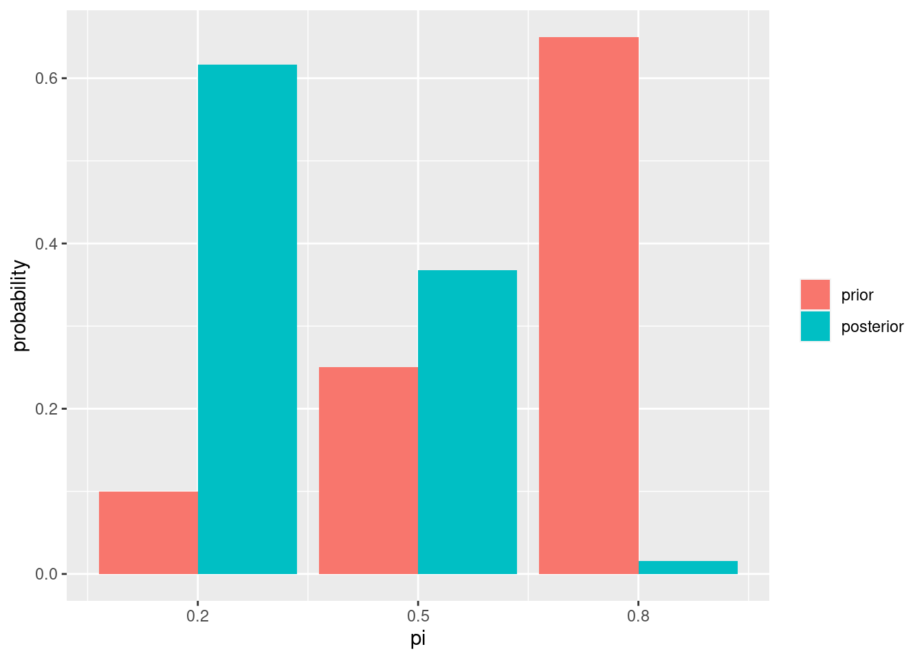

2.7.4 Posterior simulation

set.seed(84735)

sim_results <- 
  tibble(pi = sample(pi, 10000, replace = TRUE, prob = prior_prob)) |> 
  rowwise() |> 
  mutate(games_won = rbinom(1, 6, pi)) |> 
  filter(games_won == 1) |> 
  tabyl(pi) |> 
  rename(posterior_sim = percent) |> 
  mutate(posterior = posterior_prob)

sim_results |> 
  select(-n) |> 
  adorn_pct_formatting() |> 
  gt() |> 
  cols_width(1 ~ px(50), everything() ~ px(120)) |> 
  tab_header("Simulating the posterior probabilities")

Simulating the posterior probabilities
pi	posterior_sim	posterior
0.2	60.4%	61.7%
0.5	37.8%	36.8%
0.8	1.8%	1.6%