13.1 The logistic regression model
# Load packages
library(bayesrules)
library(rstanarm)
library(bayesplot)
library(tidyverse)
library(tidybayes)
library(broom.mixed)
Load and process the data
data(weather_perth)
weather <- weather_perth %>%
  select(day_of_year, raintomorrow, humidity9am, humidity3pm, raintoday)

weather %>% head
## # A tibble: 6 × 5
## day_of_year raintomorrow humidity9am humidity3pm raintoday
## <dbl> <fct> <int> <int> <fct>
## 1 45 No 55 44 No
## 2 11 No 43 16 No
## 3 261 Yes 62 85 No
## 4 347 No 53 46 No
## 5 357 No 65 51 No
## 6 254 No 84 59 YesPredict raintomorrow:
\[Y=\left\{\begin{matrix} 1 & \text{rain tomorrow}\\ 0 & \text{ otherwise} \end{matrix}\right.\]
13.1.1 Definition of Odds & probability
odds: the probability that the event happens relative to the probability that it doesn’t happen.
\[\pi \epsilon [0,1]\]
\[odds=\frac{\pi}{1-\pi} \epsilon [0,\infty)\]
\[\pi=\frac{odds}{1+odds}\]
To predict raintomorrow What’s an appropriate model structure for the data?
- Bernoulli (or, equivalently, Binomial with 1 trial)
- Gamma
- Beta
What values can \(Y_i\) take and what probability models assume this same set of values?
The Bernoulli probability model is the best candidate for the data, given that \(Y_i\) is a discrete variable which can only take two values, 0 or 1:
\[Y_i|\pi_i \sim Bern(\pi_i)\] \[E(Y_i|\pi_i)=\pi_i\]
The logistic regression model specify how the expected value of rain \(\pi_i\) depends upon predictor \(X_{i1}\):
\[g(\pi_i)=\beta_0+\beta_1 X_{i1}\]
\(\pi_i\) depends upon predictor \(X_{i1}\) through the:
\[g(\pi_i)=log(\pi_i/(1-\pi_i))\]
\[\frac{\pi_i}{1-\pi_i}=e^{\beta_0+\beta_1 X_{i1}}\]
\[\pi_i=\frac{e^{\beta_0+\beta_1 X_{i1}}}{1+e^{\beta_0+\beta_1 X_{i1}}}\] \(\beta_0\) is when all predictors are 0 \(\beta_1=log(odds_{x+1})-log(odds_x)\) \(e^{\beta_1}=\frac{odds_{x+1}}{1+odds_x}\)
\[log(odds)=log(\frac{\pi}{1-\pi})=\beta_0+\beta_1 X_{1}+...+\beta_p X_p\]
weather <- weather_perth %>%
  select(day_of_year, raintomorrow,
         humidity9am, humidity3pm, raintoday)

weather %>%head
## # A tibble: 6 × 5
## day_of_year raintomorrow humidity9am humidity3pm raintoday
## <dbl> <fct> <int> <int> <fct>
## 1 45 No 55 44 No
## 2 11 No 43 16 No
## 3 261 Yes 62 85 No
## 4 347 No 53 46 No
## 5 357 No 65 51 No
## 6 254 No 84 59 YesBased on assumptions that it will rain tomorrow with a 20% chance.
weather%>%
  count(raintomorrow)%>%
  mutate(prop=n/sum(n)*100)
## # A tibble: 2 × 3
## raintomorrow n prop
## <fct> <int> <dbl>
## 1 No 814 81.4
## 2 Yes 186 18.6weather%>%
count(raintomorrow)%>%
mutate(prop=n/sum(n)*100)%>%
ggplot(aes(x="",prop,fill=raintomorrow))+
geom_bar(stat="identity", width=1)+
coord_polar("y", start=0)+
theme_void()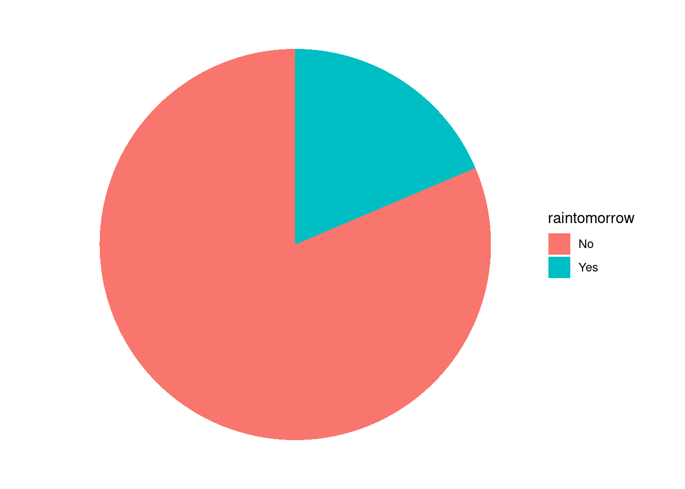
\[\pi= 0.2\]
Assumptions:
- on an average day, there’s a roughly 20% chance of rain.
- the chance of rain increases when preceded by a day with high humidity or rain.
weather %>%
  ggplot()+
  geom_line(aes(day_of_year,humidity9am),color="steelblue",linewidth=0.5)+
  geom_line(aes(day_of_year,humidity3pm),color="pink",linewidth=0.5)+
  geom_smooth(aes(day_of_year,humidity9am),color="steelblue")+
  geom_smooth(aes(day_of_year,humidity3pm),color="pink")+
  facet_wrap(vars(raintomorrow))+
  labs(title="raintomorrow?")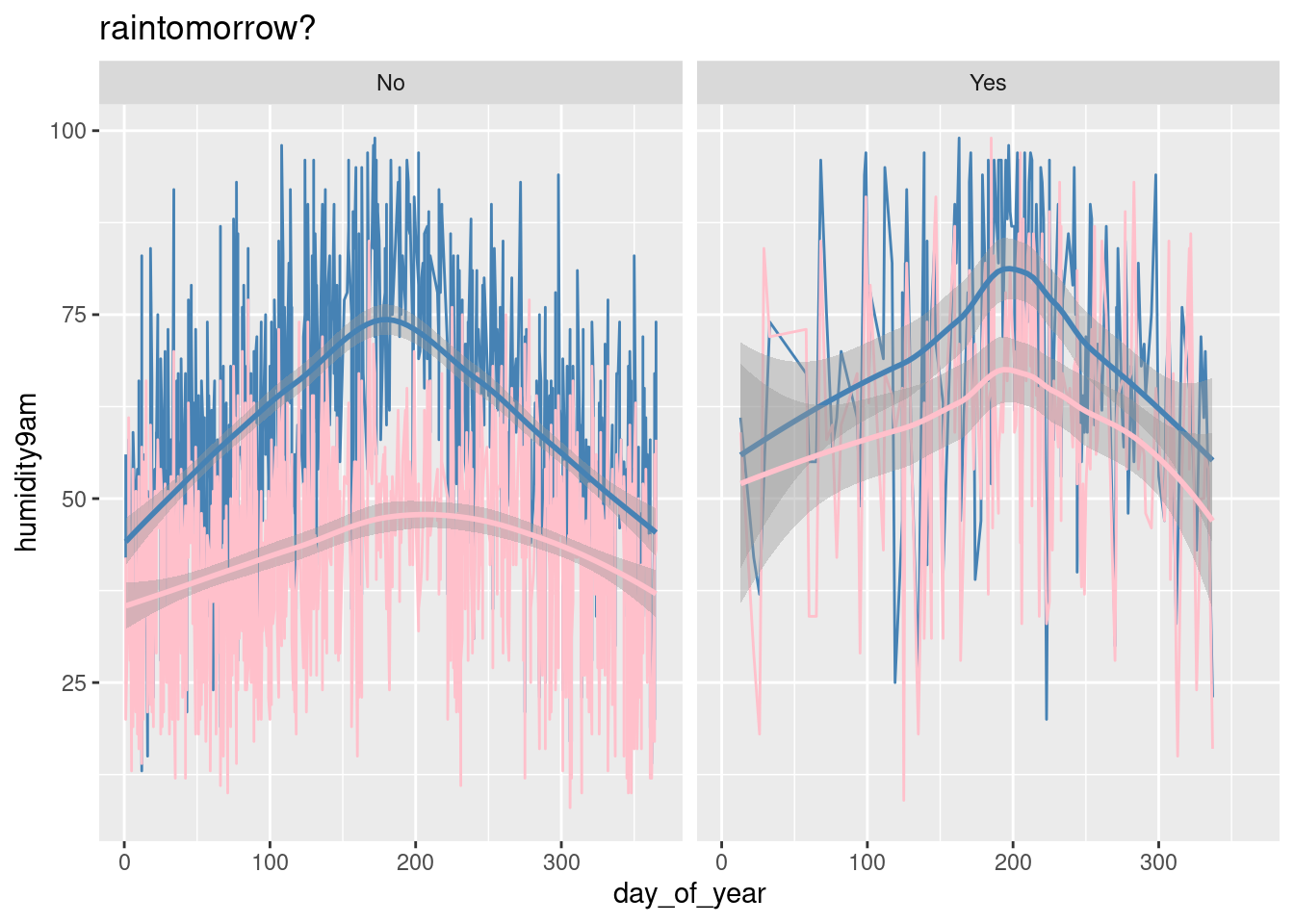
weather%>%
  ggplot(aes(raintomorrow,color=raintomorrow))+
  geom_density()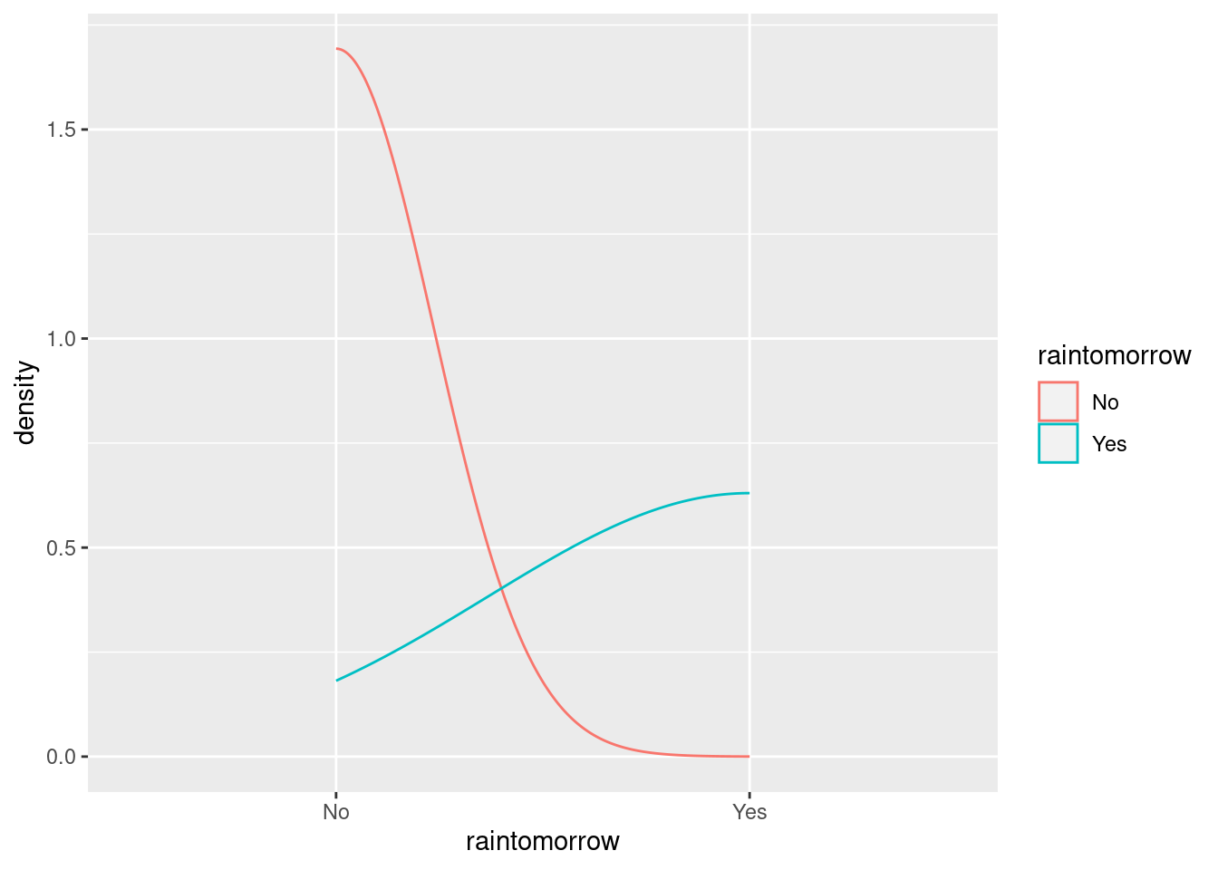
Model specification
- Data
\[Y_i|\beta_0,\beta_1 \sim^{ind} Bern(\pi_i)\] \[log(\frac{\pi_i}{1-\pi_i})=\beta_0+\beta_1 X_{i1}\]
Based on the assumption that it will rain with a 20% chance, the log odds is about -1.4. This is a centered value of a range.
log(0.2/(1-0.2))## [1] -1.386294\[log(\frac{\pi_i}{1-\pi_i}) \approx -1.4\]
13.1.2 Specifying the priors:
13.1.2.1 Beta 0 centered (\(\beta_{0c}\))
\[\beta_{0c} \sim N(\mu,\sigma)\]
The range takes consideration that it cannot go below zero, the chance of not rain has a probability of 0. And so it cannot be more than 1. Probability range: [0,1].
We are talking about logs:
log(1)## [1] 0Zero is the upper value of the range, for a max value probability of 1:
exp(log(1))## [1] 1Range: [? , 0]
\[-1.4 + 2x=0\]
x=1.4/2
x
## [1] 0.7-1.4 + 2*0.7;## [1] 0-1.4 - 2*0.7## [1] -2.8Range: (-2.8,0]
\[\beta_{0c} \sim N(-1.4,0.7^2)\]
The odds of rain on an average day could be somewhere between 0.06 and 1:
exp(-2.8);exp(0)## [1] 0.06081006## [1] 1\[(e^{-2.8},e^0) \approx (0.06,1)\]
The probability of rain on an average day could be somewhere between 0.057 and 0.50:
0.06/(1+0.06);## [1] 0.056603771/(1+1)## [1] 0.5\[(\frac{0.06}{1+0.06},\frac{1}{(1+1)}) \approx (0.057,0.5)\]
13.1.2.2 Beta 1 (\(\beta_1\))
\[\beta_1 \sim N(\mu,\sigma)\]
With the \(\beta_1\) we want to identify if the chance of rain increases when preceded by a day with high humidity.
Our range in this case has a lower limit of zero, and we estimate the upper limit to be 0.14: Range [0, 0.14]
\[(e^0,e^{0.14}) \approx (1,1.150)\]
The central value for this range is 0.07:
(0+0.14)/2## [1] 0.07Calculate the \(\sigma\) value:
\[0.07 + 2x = 0.14\]
x1= (0.14-0.07)/2
x1
## [1] 0.035So, the Normal distribution parameters are:
- \(\mu = 0.07\)
- \(\sigma=0.035\)
\[\beta_{1} \sim N(0.07,0.035^2)\]
p1<- plot_normal(mean = -1.4, sd = 0.7) +
  labs(x = "beta_0c", y = "pdf")
p2 <- plot_normal(mean = 0.07, sd = 0.035) +
  labs(x = "beta_1", y = "pdf")
library(patchwork)
p1|p2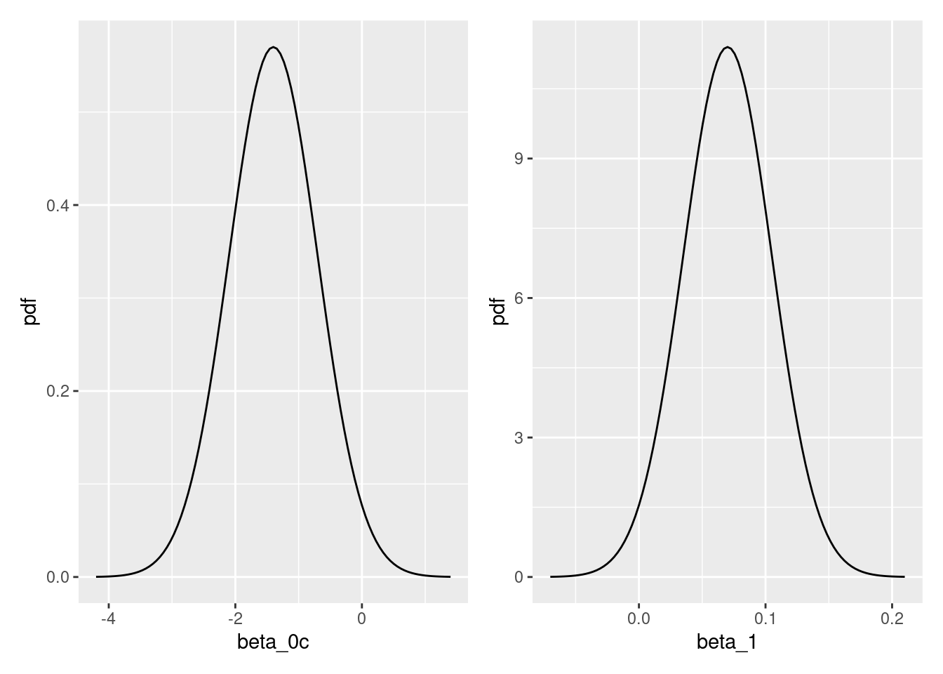
We simulate 20,000 prior plausible pairs of \(\beta_{0c}\) and \(\beta_1\) to describe a prior plausible relationship between the probability of rain tomorrow and today’s 9 a.m. humidity:
Run a prior simulation:
prior_PD = TRUErain_model_prior <- stan_glm(raintomorrow ~ humidity9am,
data = weather,
family = binomial,
prior_intercept = normal(-1.4, 0.7),
prior = normal(0.07, 0.035),
chains = 4, iter = 5000*2, seed = 84735,
prior_PD = TRUE)
rain_model_priorAnd plot just 100 of them:
add_fitted_draws(rain_model_prior, n = 100) set.seed(84735)
# Plot 100 prior models with humidity
weather %>%
add_fitted_draws(rain_model_prior, n = 100) %>%
ggplot(aes(x = humidity9am, y = raintomorrow)) +
geom_line(aes(y = .value, group = .draw), size = 0.1)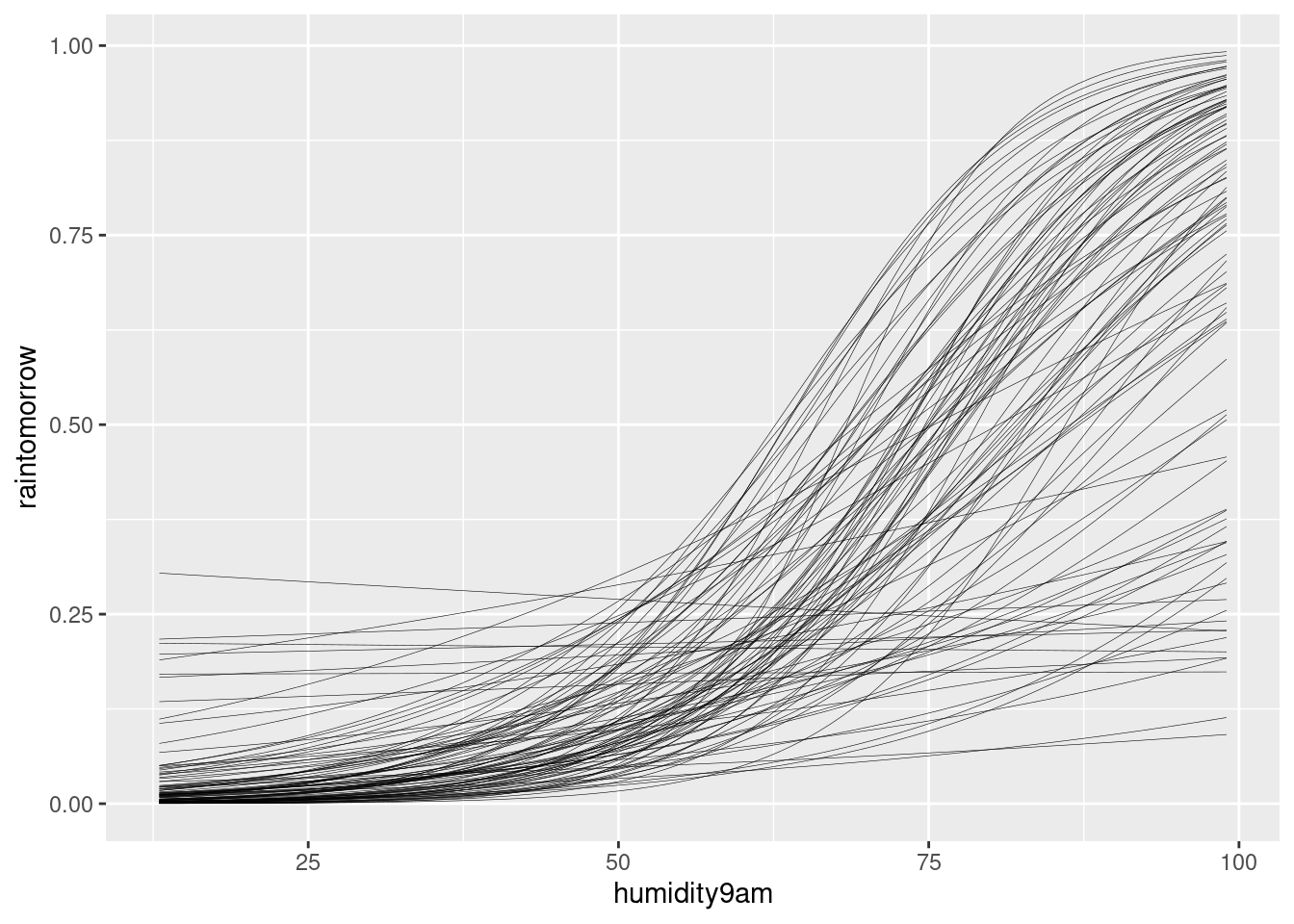
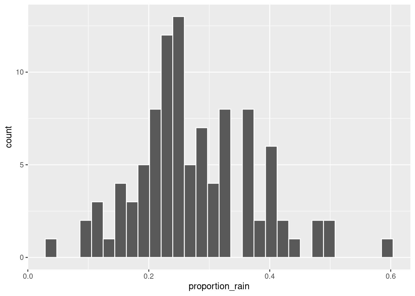
# Plot the observed proportion of rain in 100 prior datasets
weather %>%
  add_predicted_draws(rain_model_prior, n = 100) %>%
  group_by(.draw) %>%
  summarize(proportion_rain = mean(.prediction == 1)) %>%
  ggplot(aes(x = proportion_rain)) +
    geom_histogram(color = "white")