3.11 Simulating the Beta-Binomial

• Here we are going to simulate the posterior model of Michelle’s support \(\pi\). We begin by simulating 10,000 values of \(\pi\) from Beta(45,55) prior using rbeta() and, subsequently, a potential Bin(50,\(\pi\)) poll result Y from each \(\pi\) using rbinom()

• The resulting 10,000 pairs of \(\pi\) and Y values are shown below. In general, the greater Michelle’s support, the better her poll results tend to be. Further, the highlighted pairs illustrate that the eventual observed poll result, Y=30 of 50 polled voters supported Michelle, would most likely arise if her underlying support \(\pi\) were somewhere in the range from 0.4 to 0.6.

michelle_sim <- data.frame(pi = rbeta(10000,45,55)) |> 
  mutate(y=rbinom(10000,size=50,prob=pi))

ggplot(data=michelle_sim,aes(x=pi, y=y))+
  geom_point(aes(color=(y==30)),size=0.1)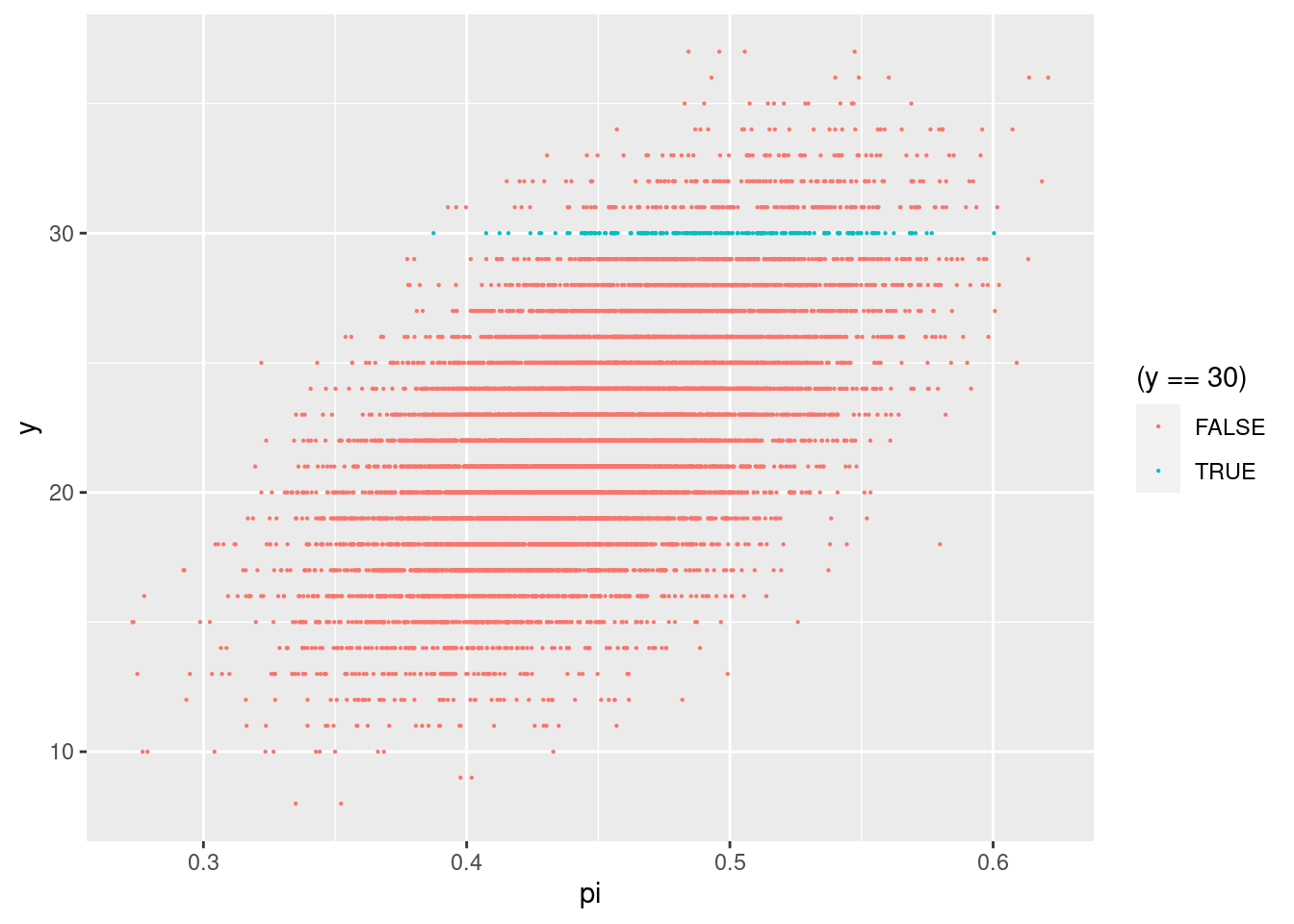

• Separate out from the simulation the results that match your new data where 30 out of 50 are supporting Michelle.

# Keep the simulated pairs that match your data

michelle_posterior <- michelle_sim |> 
  filter(y==30)

head(michelle_posterior)

##          pi  y
## 1 0.5303663 30
## 2 0.5101525 30
## 3 0.5288202 30
## 4 0.4529095 30
## 5 0.4955068 30
## 6 0.4828890 30