13.4 Model evaluation

1. How fair is the model?
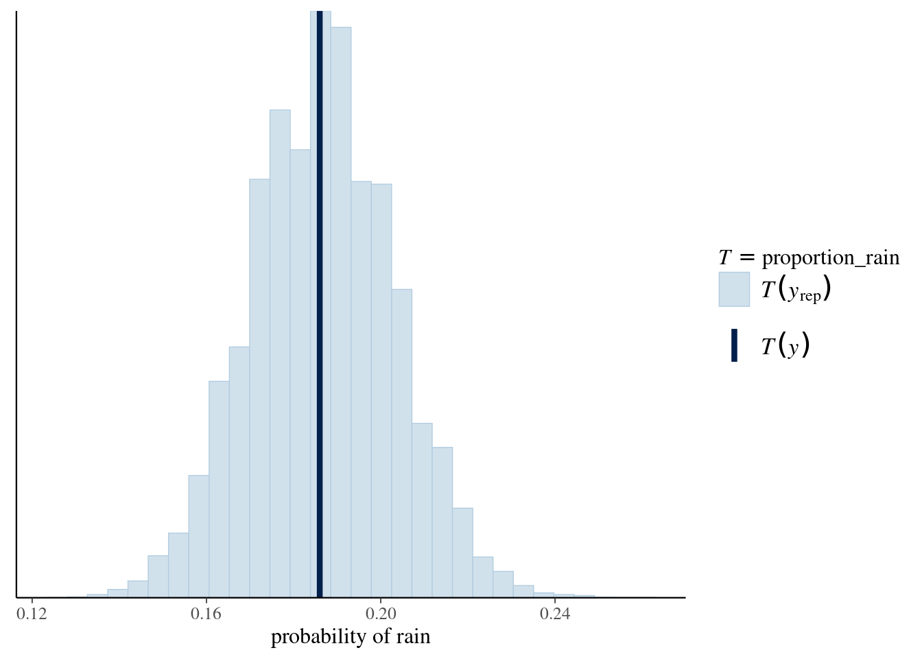
2. How wrong is the model?
3. How accurate are the model’s posterior classifications?

proportion_rain <- function(x){mean(x == 1)}

pp_check(rain_model_1, 
         #nreps = 100,
         plotfun = "stat", 
         stat = "proportion_rain") + 
  xlab("probability of rain")

Evaluate the rain_model_1 classifications:

set.seed(84735)
rain_pred_1 <- posterior_predict(rain_model_1, newdata = weather)
dim(rain_pred_1)

## [1] 20000  1000

weather_classifications <- weather %>% 
  mutate(rain_prob = colMeans(rain_pred_1),
         rain_class_1 = as.numeric(rain_prob >= 0.5)) %>% 
  select(humidity9am, rain_prob, rain_class_1, raintomorrow)

weather_classifications%>%head

## # A tibble: 6 × 4
##   humidity9am rain_prob rain_class_1 raintomorrow
##         <int>     <dbl>        <dbl> <fct>       
## 1          55    0.122             0 No          
## 2          43    0.0739            0 No          
## 3          62    0.163             0 Yes         
## 4          53    0.116             0 No          
## 5          65    0.186             0 No          
## 6          84    0.362             0 No

13.4.1 Confusion matrix

weather_classifications %>% 
  janitor::tabyl(raintomorrow, rain_class_1) %>% 
  janitor::adorn_totals(c("row", "col"))

##  raintomorrow   0  1 Total
##            No 803 11   814
##           Yes 172 14   186
##         Total 975 25  1000

set.seed(84735)
classification_summary(model = rain_model_1, 
                       data = weather, 
                       cutoff = 0.5)

## $confusion_matrix
##    y   0  1
##   No 803 11
##  Yes 172 14
## 
## $accuracy_rates
##                            
## sensitivity      0.07526882
## specificity      0.98648649
## overall_accuracy 0.81700000

Changing cutoff to 0.2 the sensitivity jumped from 7.53% to 63.98%, and the true negative rate dropped from 98.65% to 71.25%.

set.seed(84735)
classification_summary(model = rain_model_1, 
                       data = weather, 
                       cutoff = 0.2)

## $confusion_matrix
##    y   0   1
##   No 580 234
##  Yes  67 119
## 
## $accuracy_rates
##                           
## sensitivity      0.6397849
## specificity      0.7125307
## overall_accuracy 0.6990000

set.seed(84735)
cv_accuracy_1 <- classification_summary_cv(
  model = rain_model_1, 
  data = weather, 
  cutoff = 0.2, 
  k = 10)