12.2 Normal Distribution

If we follow from previous chapters, our model looks like

$$Y_{i} | \beta_{0}, \beta_{1}, \beta_{2}, \beta_{3}, \sigma \sim N(\mu_{i}, \sigma^{2})$$

with

$$\mu_{i} = \beta_{0} + \beta_{1}X_{i1} + \beta_{2}X_{i2} + \beta_{3}X_{i3}$$

12.2.1 Exploratory Data Visualization

ggplot(equality, aes(x = laws)) + 
  geom_histogram(color = "white", breaks = seq(0, 160, by = 10))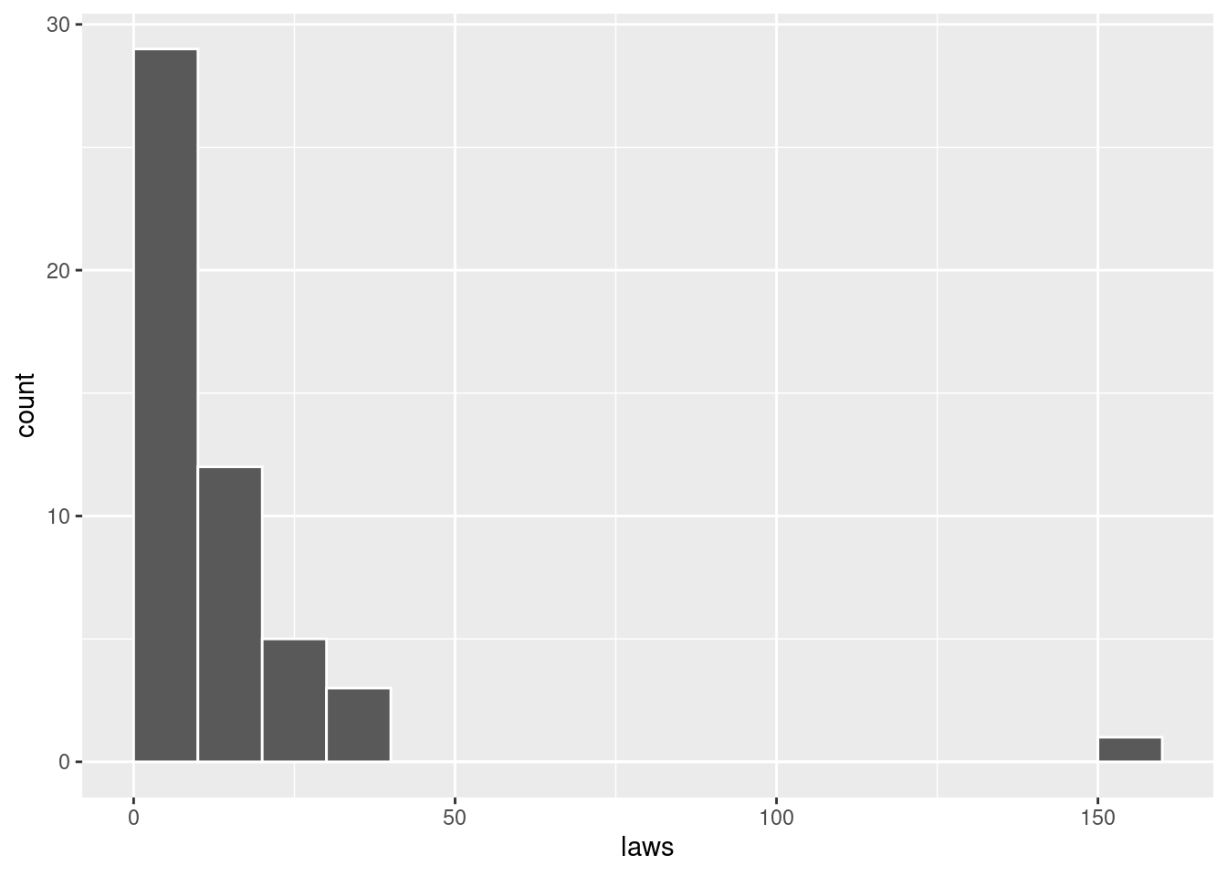

12.2.2 Outlier

# Identify the outlier
equality %>% 
  filter(laws == max(laws))

## # A tibble: 1 × 6
##   state      region gop_2016  laws historical percent_urban
##   <fct>      <fct>     <dbl> <dbl> <fct>              <dbl>
## 1 california west       31.6   155 dem                   95

# Remove the outlier
equality <- equality %>% 
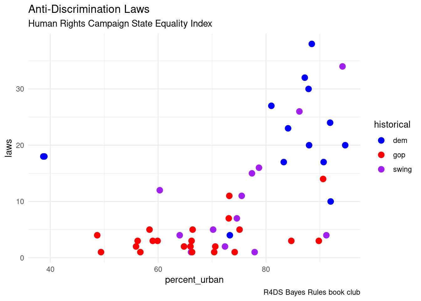
  filter(state != "california")

12.2.3 Predictor Variables

ggplot(equality, aes(y = laws, x = percent_urban, color = historical)) + 
  geom_point(size = 3) +
  labs(title = "Anti-Discrimination Laws",
       subtitle = "Human Rights Campaign State Equality Index",
       caption = "R4DS Bayes Rules book club") +
  scale_color_manual(values = c("blue", "red", "purple")) +
  theme_minimal()