14.3 One Categorical Predictor

Suppose an Antarctic researcher comes across a penguin that weighs less than 4200g with a 195mm-long flipper and 50mm-long bill. Our goal is to help this researcher identify the species of this penguin: Adelie, Chinstrap, or Gentoo

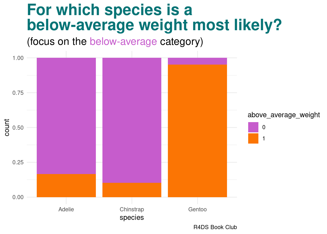
image code

penguins |>
  drop_na(above_average_weight) |>
  ggplot(aes(fill = above_average_weight, x = species)) + 
  geom_bar(position = "fill") + 
  labs(title = "<span style = 'color:#067476'>For which species is a<br>below-average weight most likely?</span>",
       subtitle = "(focus on the <span style = 'color:#c65ccc'>below-average</span> category)",
       caption = "R4DS Book Club") +
  scale_fill_manual(values = c("#c65ccc", "#fb7504")) +
  theme_minimal() +
  theme(plot.title = element_markdown(face = "bold", size = 24),
        plot.subtitle = element_markdown(size = 16))

14.3.1 Recall: Bayes Rule

$$f(y|x_{1}) = \frac{\text{prior}\cdot\text{likelihood}}{\text{normalizing constant}} = \frac{f(y) \cdot L(y|x_{1})}{f(x_{1})}$$ where, by the Law of Total Probability,

$$\begin{array}{rcl} f(x_{1} & = & \displaystyle\sum_{\text{all } y'} f(y')L(y'|x_{1}) \\ ~ & = & f(y' = A)L(y' = A|x_{1}) + f(y' = C)L(y' = C|x_{1}) + f(y' = G)L(y' = G|x_{1}) \\ \end{array}$$

over our three penguin species.

14.3.2 Calculation

penguins %>% 
  select(species, above_average_weight) %>% 
  na.omit() %>% 
  tabyl(species, above_average_weight) %>% 
  adorn_totals(c("row", "col"))

##    species   0   1 Total
##     Adelie 126  25   151
##  Chinstrap  61   7    68
##     Gentoo   6 117   123
##      Total 193 149   342

Prior probabilities:

$$f(y = A) = \frac{151}{342}, \quad f(y = C) = \frac{68}{342}, \quad f(y = G) = \frac{123}{342}$$

Likelihoods:

$$\begin{array}{rcccl} L(y = A | x_{1} = 0) & = & \frac{126}{151} & \approx & 0.8344 \\ L(y = C | x_{1} = 0) & = & \frac{61}{68} & \approx & 0.8971 \\ L(y = G | x_{1} = 0) & = & \frac{6}{123} & \approx & 0.0488 \\ \end{array}$$

Total probability:

$$f(x_{1} = 0) = \frac{151}{342}\cdot\frac{126}{151} + \frac{68}{342}\cdot\frac{61}{68} + \frac{123}{342}\cdot\frac{6}{123} = \frac{193}{342}$$

Bayes’ Rules:

$$\begin{array}{rcccccl} f(y = A | x_{1} = 0) & = & \frac{f(y = A) \cdot L(y = A | x_{1} = 0)}{f(x_{1} = 0)} = \frac{\frac{151}{342}\cdot\frac{126}{151}}{\frac{193}{342}} & \approx & 0.6528 \\ f(y = C | x_{1} = 0) & = & \frac{f(y = A) \cdot L(y = C | x_{1} = 0)}{f(x_{1} = 0)} = \frac{\frac{68}{342}\cdot\frac{61}{68}}{\frac{193}{342}} & \approx & 0.3161 \\ f(y = G | x_{1} = 0) & = & \frac{f(y = A) \cdot L(y = G | x_{1} = 0)}{f(x_{1} = 0)} = \frac{\frac{123}{342}\cdot\frac{6}{123}}{\frac{193}{342}} & \approx & 0.0311 \\ \end{array}$$

The posterior probability that this penguin is an Adelie is more than double that of the other two species