19.13 Check prediction manually

climber_df <- as.data.frame(climb_model_2)
climber_draws_Ama_Dablam <- climber_df |>
     select('(Intercept)',age, oxygen_usedTRUE,
            'b[(Intercept) peak_name:Ama_Dablam]','Sigma[expedition_id:(Intercept),(Intercept)]') |>
     rename(b_peak ='b[(Intercept) peak_name:Ama_Dablam]', sigma_exp = 'Sigma[expedition_id:(Intercept),(Intercept)]',
            B_0 = '(Intercept)')

head(climber_draws_Ama_Dablam)

        B_0         age oxygen_usedTRUE   b_peak sigma_exp
1 -1.568117 -0.05460222        5.982335 2.556797 10.682662
2 -1.642934 -0.05515428        5.534564 3.408024  6.409617
3 -1.296799 -0.05990499        6.250567 3.837433  8.373671
4 -2.153309 -0.02706937        5.822815 3.100700  7.631247
5 -2.083079 -0.05394689        6.751443 3.877804  8.072649
6 -2.595809 -0.03535885        5.731177 4.762982 12.472273

Ok for each of these 20000 draws, we compute a random expedition tweak with the appropriate sigma, and then compute the probability from the inverse logistic.

logit_draws <- climber_draws_Ama_Dablam |>
  mutate(exp_tweak = rnorm(n(),0, sqrt(sigma_exp))) |>
  mutate(without_tweak = B_0 + 30*age + oxygen_usedTRUE + b_peak,
         with_tweak =  without_tweak + exp_tweak)
 
draws_longer <- logit_draws |> pivot_longer(cols = c('without_tweak', 'with_tweak'), names_to = "tweak", values_to = "logit")

draws_longer <- draws_longer |> mutate(prob_success = invlogit(logit))

ggplot(data = draws_longer) + geom_density(mapping = aes(x=logit, color=tweak))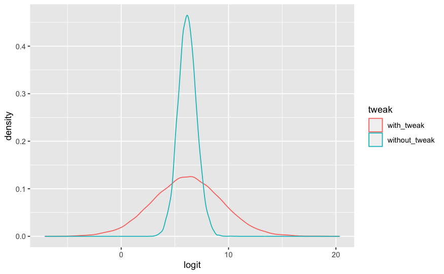

Summary statistics:

draws_longer |> group_by(tweak) |> 
  summarize(mean=mean(prob_success),
           median=median(prob_success),
           q_lower = quantile(prob_success,.1),
           q_higher = quantile(prob_success,.9),.groups = "drop")

# A tibble: 2 × 5
  tweak          mean median q_lower q_higher
  <chr>         <dbl>  <dbl>   <dbl>    <dbl>
1 with_tweak    0.952  0.998   0.885    1.00 
2 without_tweak 0.997  0.998   0.994    0.999

The expedition random tweak only effects the mean, the median is invariant for monotonic function like invlogit. But the mean is what you get if you simulate the Bernoulli event for each probability draw in the same way posterior_predict does.

\[ p_{succ} = \mathbb{E}(Y) \approx \frac{1}{N_{draws}} \sum_{draws} \pi_{draw} = \mathbb{E}(\pi) \]

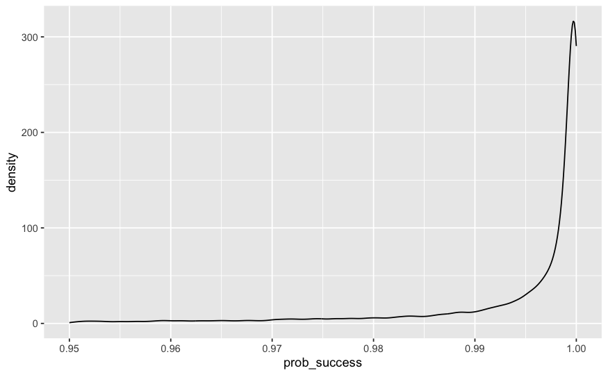
Or one could report the full posterior for \(\pi\) :

ggplot(data = draws_longer |> filter(tweak=='with_tweak')) +
  geom_density(mapping = aes(x=prob_success )) + xlim(.95,1)