9.5 Posterior simulatiion

Now we want to update our prior with data to get a posterior simulation!

# Load and plot data
library("bayesrules")
library("ggplot2")

data(bikes)

ggplot(bikes, aes(x = temp_feel, y = rides)) + 
  geom_point(size = 0.5) + 
  geom_smooth(formula = "y ~ x", method = "lm", se = FALSE) +
  labs(title = "Washington DC Bike Ridership",
       subtitle = "Fanaee-T, Hadi and Gama, Joao (2013)",
       caption = "R4DS Book Club",
       x = "what the temperature feels like (degrees Fahrenheit)",
       y = "number of bikeshare rides") +
  theme_minimal()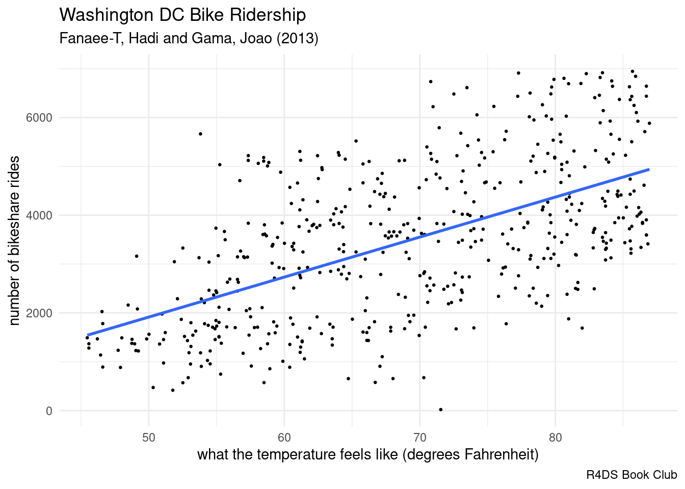

I am saving you from the triple integrals in the denominator of p 220 and we are jumping directly to MCMC! We are going to use rstanarm : Rstan + arm = applied regression models

9.5.1 Simulation via rstanarm

bike_model <- rstanarm::stan_glm(
  # data information
  rides ~ temp_feel, # <- formula syntax (as used by lm, glm etc)
  data = bikes, 
  family = gaussian, # <- we assume normal data 
  
  # Priors  
  prior_intercept = normal(5000, 1000), # centered intercept
  prior = normal(100, 40), 
  prior_aux = exponential(0.0008), #notice the aux for auxiliary more after
  
  # MCMC information
  chains = 4, iter = 5000*2, seed = 84735)

9.5.2 Simulation directly with rstan

# STEP 1: DEFINE the model
stan_bike_model <- "
  data {
    int<lower = 0> n;
    vector[n] Y;
    vector[n] X;
  }
  parameters {
    real beta0;
    real beta1;
    real<lower = 0> sigma;
  }
  model {
    Y ~ normal(beta0 + beta1 * X, sigma);
    beta0 ~ normal(-2000, 1000);
    beta1 ~ normal(100, 40);
    sigma ~ exponential(0.0008);
  }
"

# STEP 2: SIMULATE the posterior
stan_bike_sim <- 
  rstan::stan(model_code = stan_bike_model, 
       # data is structured a bit differently 
       data = list(n = nrow(bikes), Y = bikes$rides, X = bikes$temp_feel), 
       # same MCMC
       chains = 4, iter = 5000*2, seed = 84735)

The model will return 5000 x nb of chains simulation of our parameters. Rstanarm will change their name:

• \(\beta_{0} \rightarrow (intercept)\)

  • Note that this is \(\beta_{0}\) even though prior is specified for \(\beta_{0c}\)

• \(\beta_{1} \rightarrow temp\_feel\)

• But \(\sigma\) stays as \(\sigma\)

We need to check if the simulation went well for that we can?

Answer:

[X] Check the effective sample size: neff_ratio

[X] Compute rhat

[X] Examine trace plots

[X] Overlay the density plots of chains