11.2 Utilizing a categorical predictor

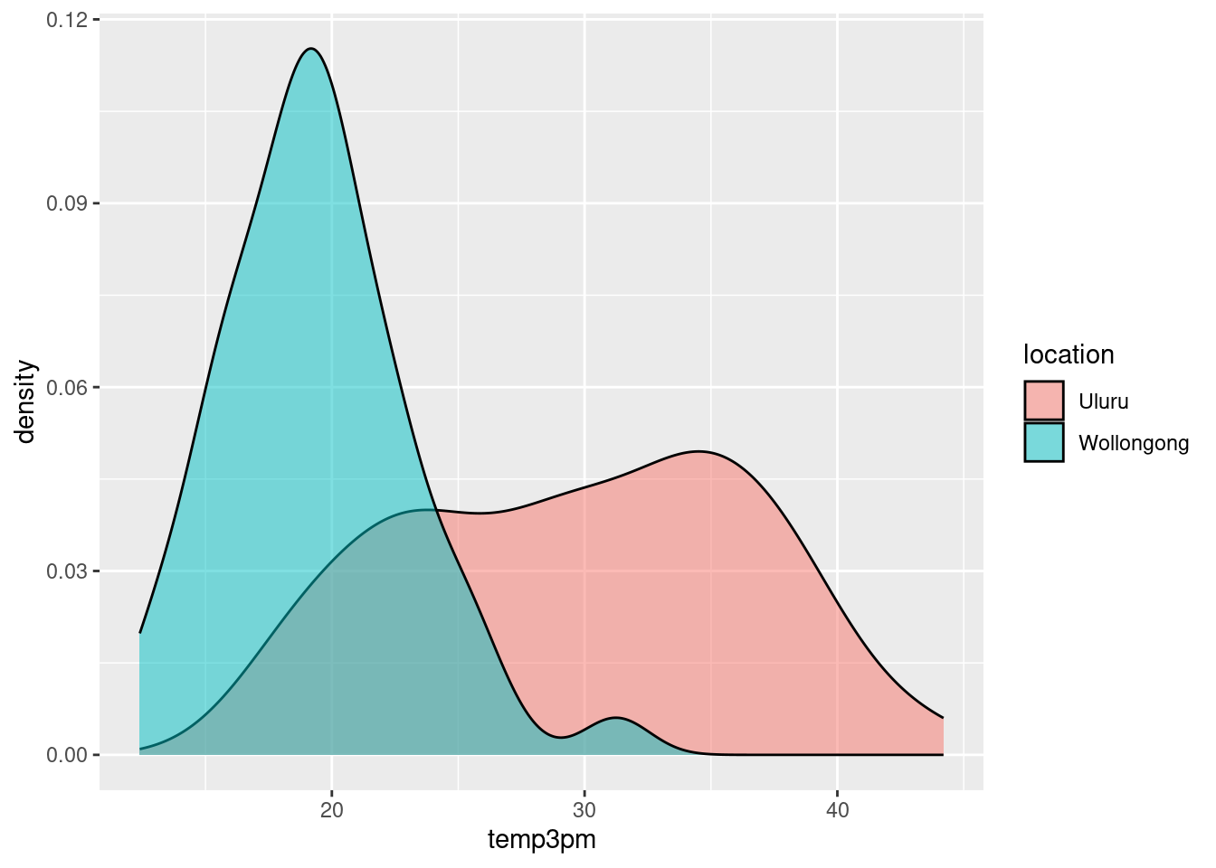
ggplot(weather_WU, aes(x = temp3pm, fill = location)) + 
  geom_density(alpha = 0.5)

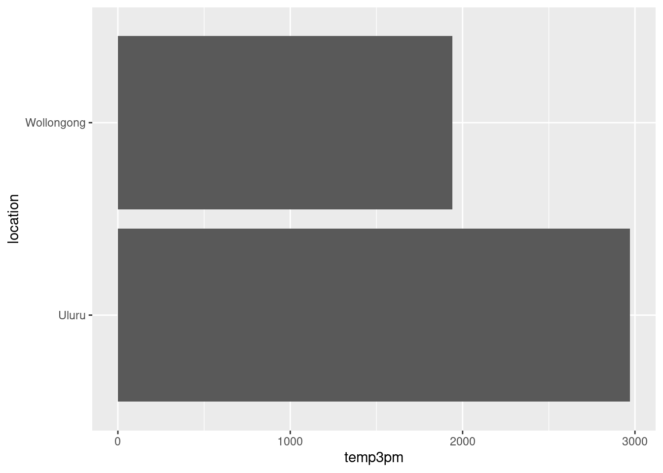
ggplot(weather_WU, aes(x=temp3pm , y=location)) + 
  geom_col()

weather_WU%>%
  group_by(location)%>%
  reframe(avg=mean(temp3pm),sd=sd(temp3pm),)

## # A tibble: 2 × 3
##   location     avg    sd
##   <fct>      <dbl> <dbl>
## 1 Uluru       29.7  6.82
## 2 Wollongong  19.4  3.66

weather_model_2 <- stan_glm(
  temp3pm ~ location,
  data = weather_WU, 
  family = gaussian,
  prior_intercept = normal(25, 5),
  
  prior = normal(0, 2.5, autoscale = TRUE), 
  prior_aux = exponential(1, autoscale = TRUE),
  
  chains = 4, iter = 5000*2, seed = 84735)

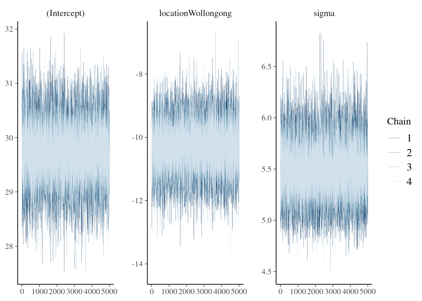
# MCMC diagnostics
mcmc_trace(weather_model_2, size = 0.1)

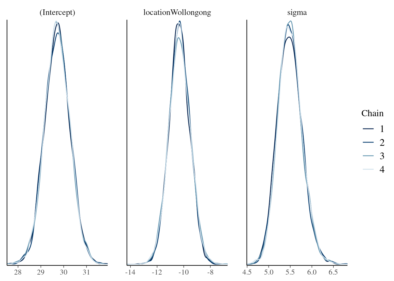
mcmc_dens_overlay(weather_model_2)

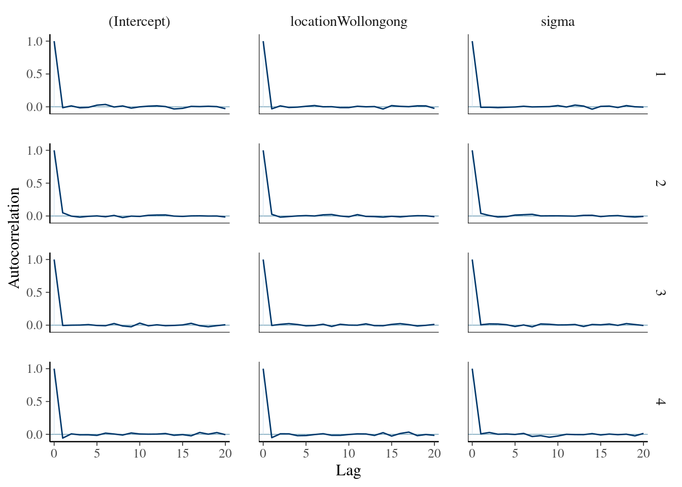
mcmc_acf(weather_model_2)

tidy(weather_model_2, effects = c("fixed", "aux"),
     conf.int = TRUE, conf.level = 0.80) %>% 
  select(-std.error)

## # A tibble: 4 × 4
##   term               estimate conf.low conf.high
##   <chr>                 <dbl>    <dbl>     <dbl>
## 1 (Intercept)           29.7     29.0      30.4 
## 2 locationWollongong   -10.3    -11.3      -9.30
## 3 sigma                  5.48     5.14      5.86
## 4 mean_PPD              24.6     23.9      25.3

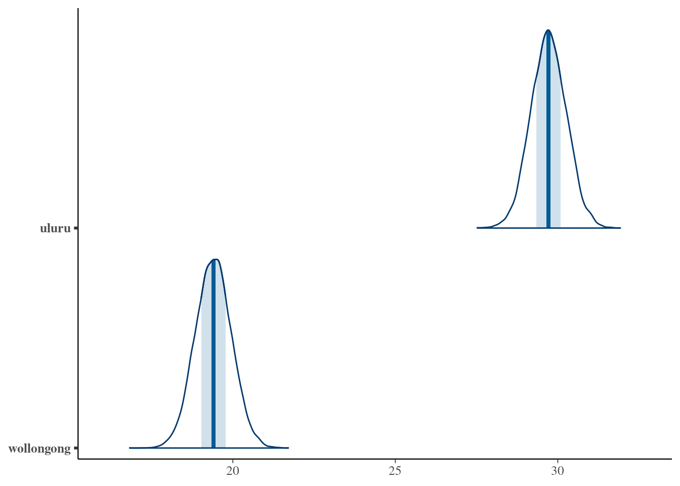
as.data.frame(weather_model_2) %>% 
  mutate(uluru = `(Intercept)`, 
         wollongong = `(Intercept)` + locationWollongong) %>% 
  mcmc_areas(pars = c("uluru", "wollongong"))