9.6 Interpreting the posterior

What we have is samples of each of the parameters.

# Posterior summary statistics
broom.mixed::tidy(bike_model, # it takes our output from rstanarm::stan_glm
                
                  # fixed is regression coef 
                  # aux is auxiliary, i.e. sigma
                  effects = c("fixed", "aux"), 
                  conf.int = TRUE, conf.level = 0.80)

# A tibble: 4 x 5
  term        estimate std.error conf.low conf.high
  <chr>          <dbl>     <dbl>    <dbl>     <dbl>
1 (Intercept)  -2194.     362.    -2656.    -1732. 
2 temp_feel       82.2      5.15     75.6      88.8
3 sigma         1281.      40.7    1231.     1336. 
4 mean_PPD      3487.      80.4    3385.     3591. 

Here we can get the posterior median relationship :

\[ -2194.24 + 82.16X \] If we want a bigger picture:

# Store the 4 chains for each parameter in 1 data frame
bike_model_df <- as.data.frame(bike_model)

# Check it out
nrow(bike_model_df)
[1] 20000
head(bike_model_df, 3)
  (Intercept) temp_feel sigma
1       -2657     88.16  1323
2       -2188     83.01  1323
3       -1984     81.54  1363

# 50 simulated model lines
bikes %>%
  tidybayes::add_fitted_draws(bike_model, n = 50) %>%
  ggplot(aes(x = temp_feel, y = rides)) +
    geom_line(aes(y = .value, group = .draw), alpha = 0.15) + 
    geom_point(data = bikes, size = 0.05)
# [code not executed for run-time consideration]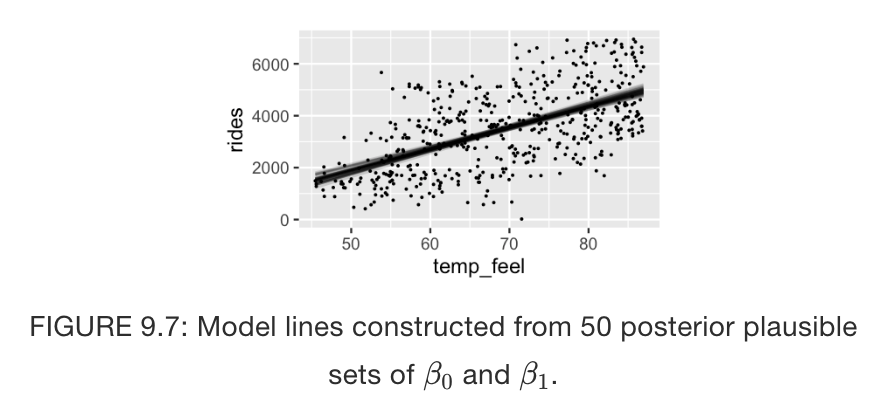

Figure 9.7

Quiz: Do we have ample posterior evidence that there’s a positive association between ridership and temperature ?

Answer:

• Visual evidence : 50 or more posterior scenarios that display positive relationship

• Numerical evidence from credible interval:

  • 80% CI for \(\beta_{1}\) range from 75.6 to 88.8

• Numerical evidence from posterior probability

# Tabulate the beta_1 values that exceed 0
bike_model_df %>% 
  mutate(exceeds_0 = temp_feel > 0) %>% 
  tabyl(exceeds_0)
# imitate hypothesis test (null: coefficient = 0)
 exceeds_0     n percent
      TRUE 20000     100