12.4 Poisson Regression

$$Y_{i} | \lambda_{i} \sim \text{Pois}(\lambda_{i})$$

• expected value: $\text{E}(Y_{i}|\lambda_{i}) = \lambda_{i}$
• variance: $\text{Var}(Y_{i}|\lambda_{i}) = \lambda_{i}$
• does $\lambda_{i} = \beta_{0} + \beta_{1}X_{i1} + \beta_{2}X_{i2} + \beta_{3}X_{i3}$?

equality |>
  ggplot(aes(x = percent_urban, y = laws, group = historical)) +
  geom_smooth(aes(color = historical),
              formula = "y ~ x",
              linewidth = 3,
              method = "lm",
              se = FALSE) +
  labs(title = "Anti-Discrimination Laws",
       subtitle = "Human Rights Campaign State Equality Index",
       caption = "R4DS Bayes Rules book club") +
  scale_color_manual(values = c("blue", "red", "purple")) +
  theme_minimal() +
  xlim(0, 100)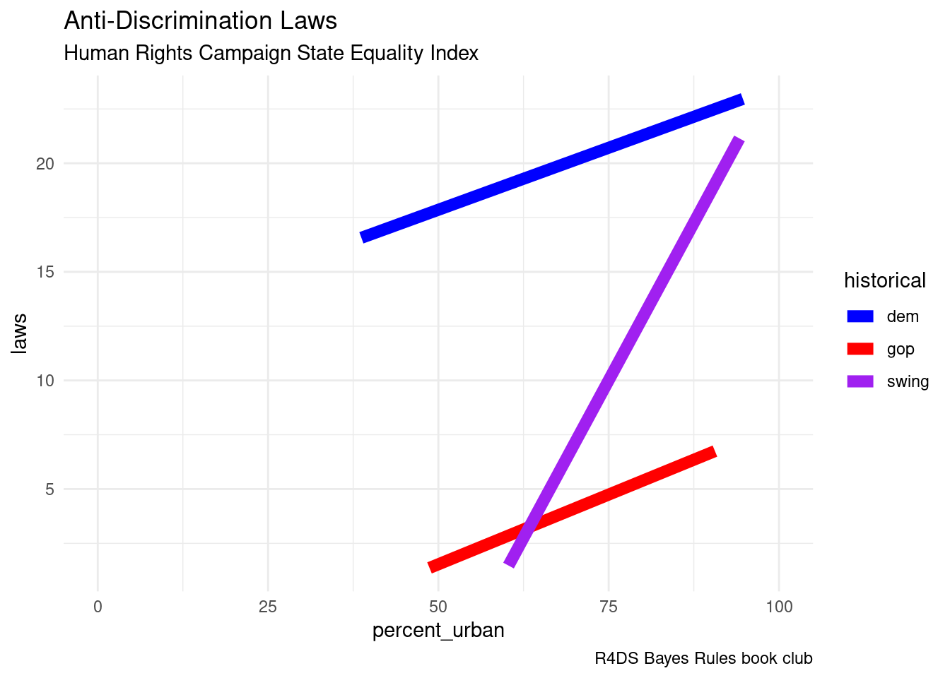

• observe that some of the predicted counts (for number of laws) are negative!

12.4.1 Log-Link Function

$$Y_{i} | \beta_{0}, \beta_{1}, \beta_{2}, \beta_{3}, \sigma \sim \text{Pois}(\lambda_{i})$$

with

$$\log(\lambda_{i}) = \beta_{0} + \beta_{1}X_{i1} + \beta_{2}X_{i2} + \beta_{3}X_{i3}$$ or $$\lambda_{i} = e^{\beta_{0} + \beta_{1}X_{i1} + \beta_{2}X_{i2} + \beta_{3}X_{i3}}$$

12.4.2 rstan

equality_model_prior <- stan_glm(laws ~ percent_urban + historical, 
                                 data = equality, 
                                 family = poisson,
                                 prior_intercept = normal(2, 0.5),
                                 prior = normal(0, 2.5, autoscale = TRUE), 
                                 chains = 4, iter = 5000*2, seed = 84735, 
                                 prior_PD = TRUE)

12.4.3 Poisson Regression Assumptions

• Structure of the data: Conditioned on predictors $X$, the observed data $Y_i$ on case $i$ is independent of the observed data on any other case $j$.
• Structure of the variable $Y$: Response variable $Y$ has a Poisson structure, i.e., is a discrete count of events that happen in a fixed interval of space or time.
• Structure of the relationship: The logged average $Y$ value can be written as a linear combination of the predictors $$\log(\lambda_{i}) = \beta_{0} + \beta_{1}X_{i1} + \beta_{2}X_{i2} + \beta_{3}X_{i3}$$
• Structure of the variability in $Y$: A Poisson random variable $Y$ with rate $\lambda$ has equal mean and variance, $\text{E}(Y)=\text{Var}(Y)=\lambda$. Thus, conditioned on predictors $X$, the typical value of $Y$ should be roughly equivalent to the variability in $Y$. As such, the variability in $Y$ increases as its mean increases.