8.5 Posterior analysis with MCMC

Markov chains of \(\pi\) for 10,000 iterations each.

8.5.1 Posterior simulation

library(rstan)
# STEP 1: DEFINE the model
art_model <- "
  data {
    int<lower = 0, upper = 100> Y;
  }
  parameters {
    real<lower = 0, upper = 1> pi;
  }
  model {
    Y ~ binomial(100, pi);
    pi ~ beta(4, 6);
  }
"

# STEP 2: SIMULATE the posterior
art_sim <- stan(model_code = art_model, 
                data = list(Y = 14), 
                chains = 4,
                iter = 5000*2, 
                seed = 84735)

library(bayesplot)
# Parallel trace plots & density plots
mcmc_trace(art_sim, pars = "pi", size = 0.5) + 
  xlab("iteration")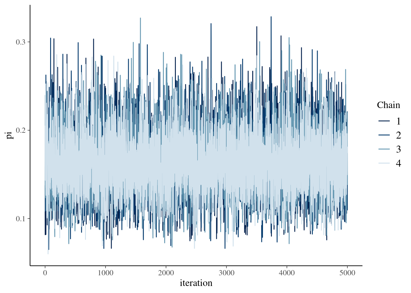

mcmc_dens_overlay(art_sim, pars = "pi")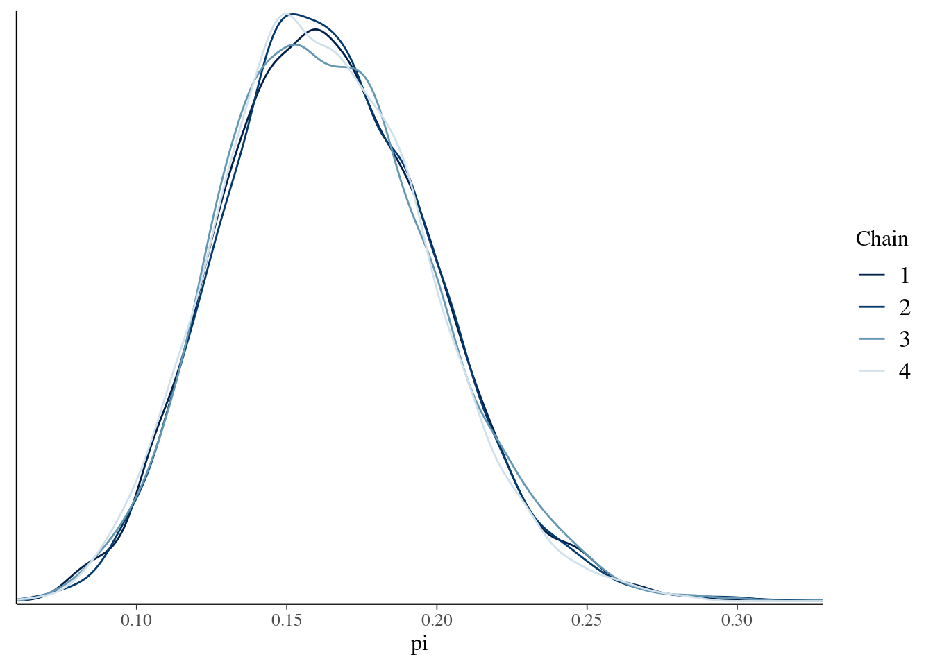

# Autocorrelation plot
mcmc_acf(art_sim, pars = "pi")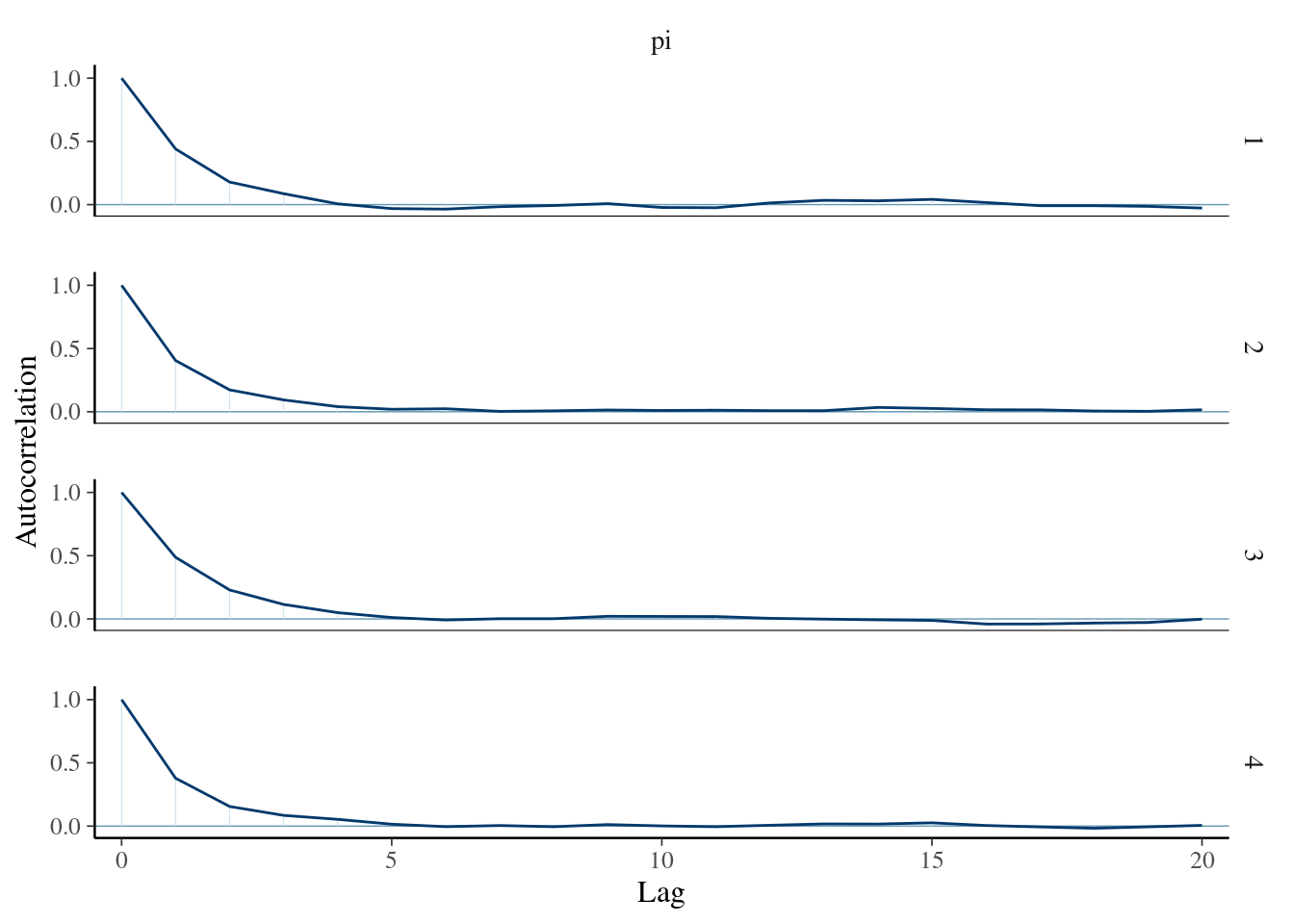

# Markov chain diagnostics
rhat(art_sim, pars = "pi")

## [1] 1.000811

neff_ratio(art_sim, pars = "pi")

## [1] 0.399955

8.5.2 Posterior estimation & hypothesis testing

Combined 20,000 Markov chain values.

# The actual Beta(18, 92) posterior
plot_beta(alpha = 18, beta = 92) + 
  lims(x = c(0, 0.35))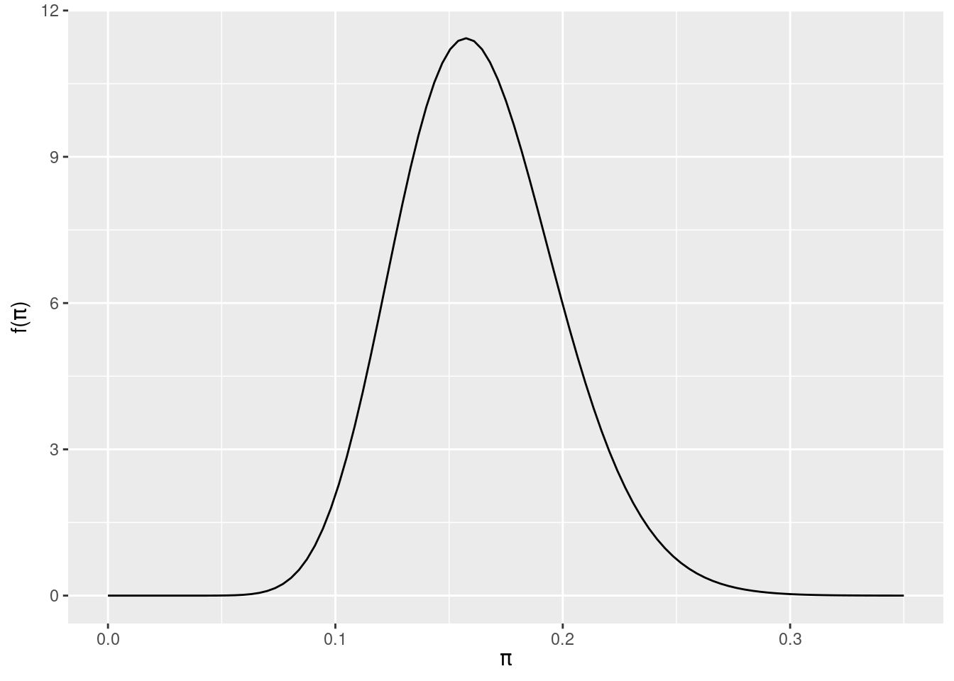

# MCMC posterior approximation
mcmc_dens(art_sim, pars = "pi") + 
  lims(x = c(0,0.35))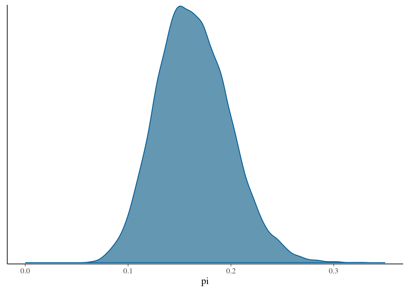

library(broom.mixed)
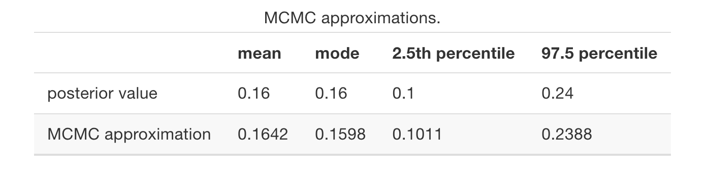
tidy(art_sim, conf.int = TRUE, conf.level = 0.95)

## # A tibble: 1 × 5
##   term  estimate std.error conf.low conf.high
##   <chr>    <dbl>     <dbl>    <dbl>     <dbl>
## 1 pi       0.162    0.0351    0.101     0.237

# Shade in the middle 95% interval
mcmc_areas(art_sim, pars = "pi", prob = 0.95)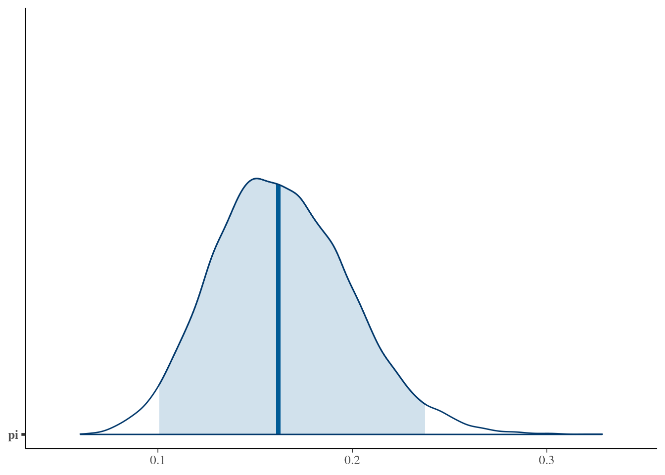

# Store the 4 chains in 1 data frame
art_chains_df <- as.data.frame(art_sim, pars = "lp__", include = FALSE)
dim(art_chains_df)

## [1] 20000     1

# Calculate posterior summaries of pi
art_chains_df %>% 
  summarize(post_mean = mean(pi), 
            post_median = median(pi),
            post_mode = sample_mode(pi),
            lower_95 = quantile(pi, 0.025),
            upper_95 = quantile(pi, 0.975))

##   post_mean post_median post_mode  lower_95  upper_95
## 1 0.1637786   0.1618674 0.1507449 0.1006319 0.2374311

Calculate summary statistics directly from the Markov chain values.

We can approximate the posterior probability \[P(\pi < 0.20 | Y =14)\]

library(janitor)
# Tabulate pi values that are below 0.20
art_chains_df %>% 
  mutate(exceeds = pi < 0.20) %>% 
  tabyl(exceeds)

##  exceeds     n percent
##    FALSE  3042  0.1521
##     TRUE 16958  0.8479

Compare results

8.5.3 Posterior prediction

Utilize the Markov chain values to approximate the posterior predictive model of \(Y'\). Repeating previous assumptions (sampling and posterior variability) and using rbinom(), we obtain:

# Set the seed
set.seed(1)

# Predict a value of Y' for each pi value in the chain
art_chains_df <- art_chains_df %>% 
  mutate(y_predict = rbinom(length(pi), 
                            size = 20, 
                            prob = pi))

# Check it out
art_chains_df %>% 
  head(3)

##           pi y_predict
## 1 0.10809936         1
## 2 0.08175123         1
## 3 0.09811126         2

# Plot the 20,000 predictions
ggplot(art_chains_df, aes(x = y_predict)) + 
  stat_count()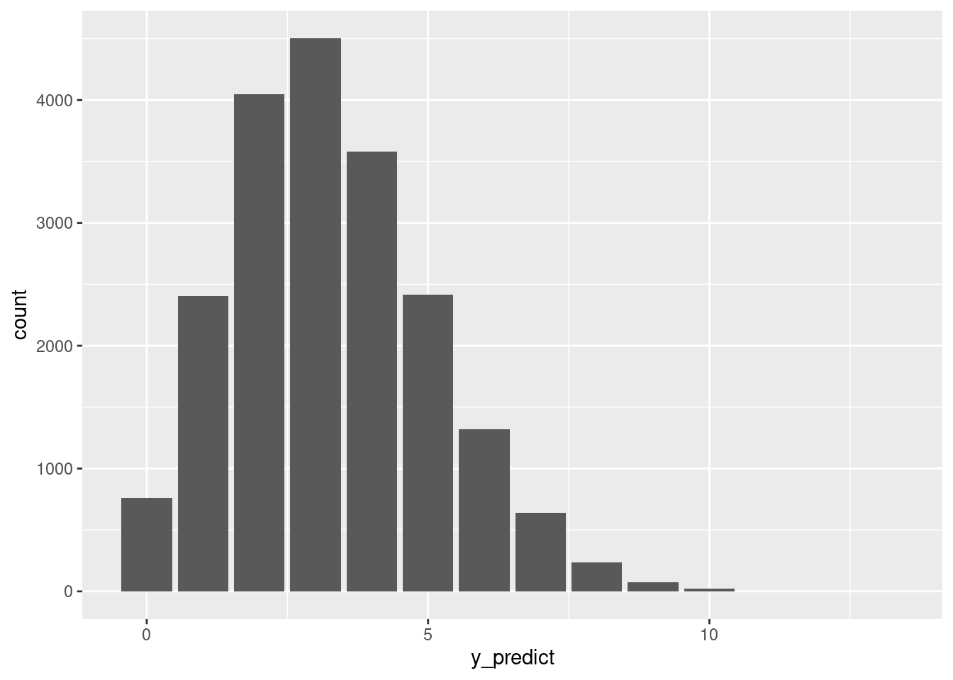

Approximate the posterior mean prediction \(E(Y'|Y=14)\) and the posterior prediction interval for \(Y'\).

art_chains_df %>% 
  summarize(mean = mean(y_predict),
            lower_80 = quantile(y_predict, 0.1),
            upper_80 = quantile(y_predict, 0.9))

##     mean lower_80 upper_80
## 1 3.2793        1        6