10.4 Our Case Study
- number of Capital Bikeshare rides: \(Y_{i}\)
- temperature on day \(i\): \(X_{i}\)
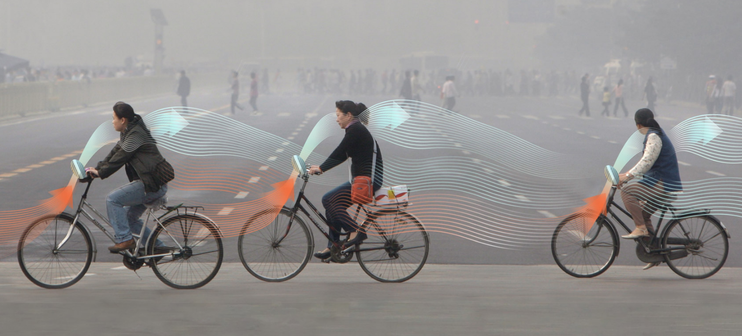
(#fig:10.2)Credits: dezeen.com
Starting from a Regression Model:
\[ Y_{i} = \beta_{0} + \beta_{1}X_{i} \]
We look for an approximation of the real mean value: estimate mean value
\[Y_{i} \approx\mu_{i}\] \[ \mu_{i} = \beta_{0} + \beta_{1}X_{i} \]
“…To turn this into a Bayesian model, we must incorporate prior models for each of the unknown regression parameters…(ct.9.1.2)”
with these model parameters:
\[ Y_{i}| \beta_{0}, \beta_{1}, \sigma \overset{ind}{\sim} N(\mu_{i}, \sigma^2) \; with \quad \mu_{i} = \beta_{0} + \beta_{1}X_{i} \]
we expect some good results as we consider 500 daily observations within a two-year period.
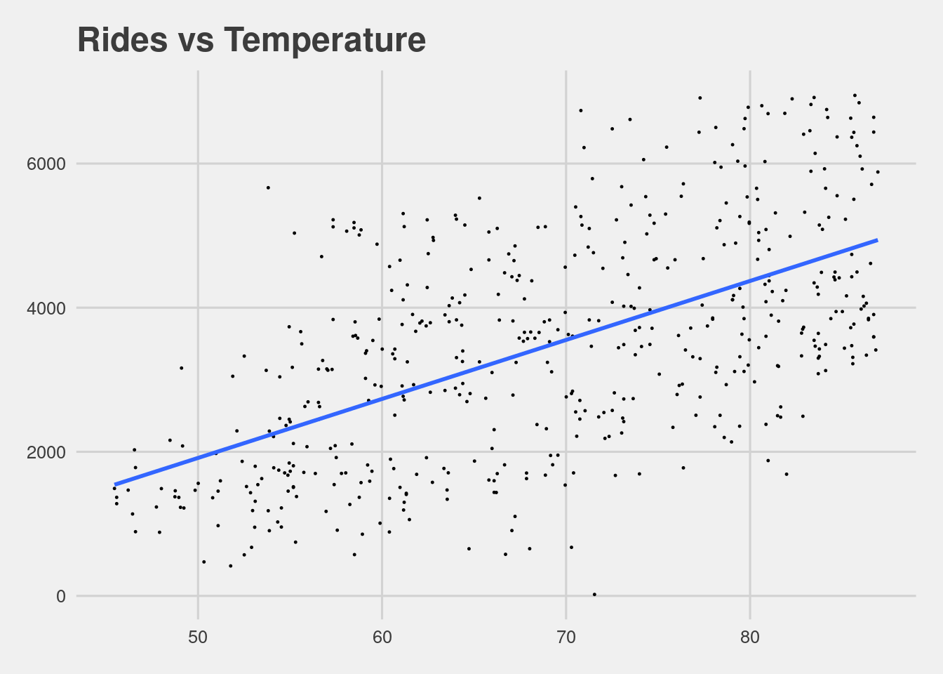
The response variable ridership \(Y\) is likely to be correlated over time with other features such as temperature \(X\).
“…today’s ridership likely tells us something about tomorrow’s ridership. Yet much of this correlation, or dependence, can be explained by the time of year and features associated with the time of year…”
“…knowing the temperature on two subsequent days may very well “cancel out” the time correlation in their ridership data…”
We are tempted to conclude:
- the temperatures in one location are independent of those in neighboring locations,
- the temperatures in one month don’t tell us about the next.
(#fig:10.3)Assumption1
It’s reasonable to assume that, in light of the temperature \(X\), ridership data \(Y\) is independent from day to day.
We are looking for a centered value of the intercept:
\[ \beta_{0c} \sim N(m_{0}, s^2_{0})= N(5000, 1000^2 ) \tag{a.}\]
\[ \beta_{1} \sim N(m_{1}, s^2_{1}) = N(100, 40^2 \tag{b.}) \] \[ \sigma\sim Exp(l) = Exp(0.0008 \tag{c.}) \]
##         date rides temp_feel
## 1 2011-01-01   654  64.72625
## 2 2011-01-03  1229  49.04645
## 3 2011-01-04  1454  51.09098
## 4 2011-01-05  1518  52.63430
## 5 2011-01-07  1362  50.79551
## 6 2011-01-08   891  46.60286
To evaluate assumptions 2 and 3 we conduct a posterior predictive check.
Our first look was at the relationship between rides and temperature, and so at the consistency of the distribution.
(#fig:10.7)Assumption 2 and 3
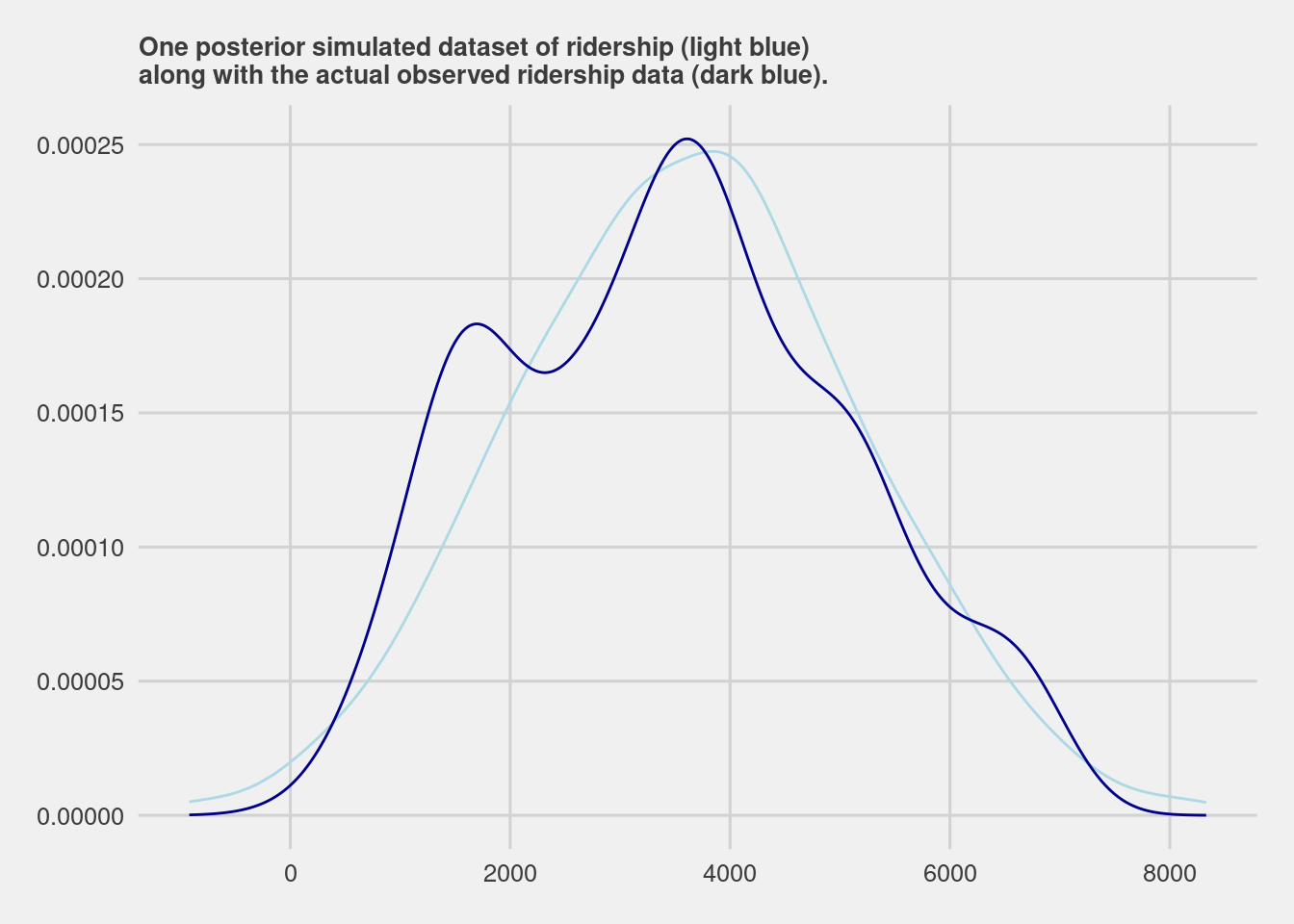
Given the combined model assumptions reasonable, the posterior model should be able to simulate ridership data very close to the original 500 rides observations.
bike_model <- rstanarm::stan_glm(
                       rides ~ temp_feel,
                       data = bikes,
                       family = gaussian,
                       prior_intercept = normal(5000, 1000),
                       prior = normal(100, 40),
                       prior_aux = exponential(0.0008),
                       chains = 4, iter = 5000*2, seed = 84735,
                       # suppress the output
                       refresh=0)
bike_model_df <- as.data.frame(bike_model)
first_set <- head(bike_model_df, 1)
first_set## (Intercept) temp_feel sigma
## 1 -2040.536 80.44231 1280.101beta_0 <- first_set$`(Intercept)`
beta_1 <- first_set$temp_feel
sigma <- first_set$sigma
set.seed(84735)
one_simulation <- bikes %>%
mutate(mu = beta_0 + beta_1 * temp_feel,
simulated_rides = rnorm(500, mean = mu, sd = sigma)) %>%
select(temp_feel, rides, simulated_rides)
one_simulation%>%head## temp_feel rides simulated_rides
## 1 64.72625 654 4020.319
## 2 49.04645 1229 1746.346
## 3 51.09098 1454 3068.930
## 4 52.63430 1518 2496.768
## 5 50.79551 1362 3065.187
## 6 46.60286 891 3735.023ggplot(one_simulation, aes(x = simulated_rides)) +
geom_density(color = "lightblue") +
geom_density(aes(x = rides), color = "darkblue")+
labs(title="One posterior simulated dataset of ridership (light blue)\nalong with the actual observed ridership data (dark blue).")+
ggthemes::theme_fivethirtyeight()+
theme(plot.title = element_text(size=10))