16.2 Complete pooled model
Notations:
\(j\) will indicate artist, \(j \in {1, 2 ..., 44}\)
\(i\) will indicate song for artist \(j\)
\(n_j\) Number of song we have for artist \(j\)
Example: Mia X, the first artist in our data set, has 4 songs -> \(n_1 = 4\)
ggplot(spotify, aes(x = popularity)) +
  geom_density()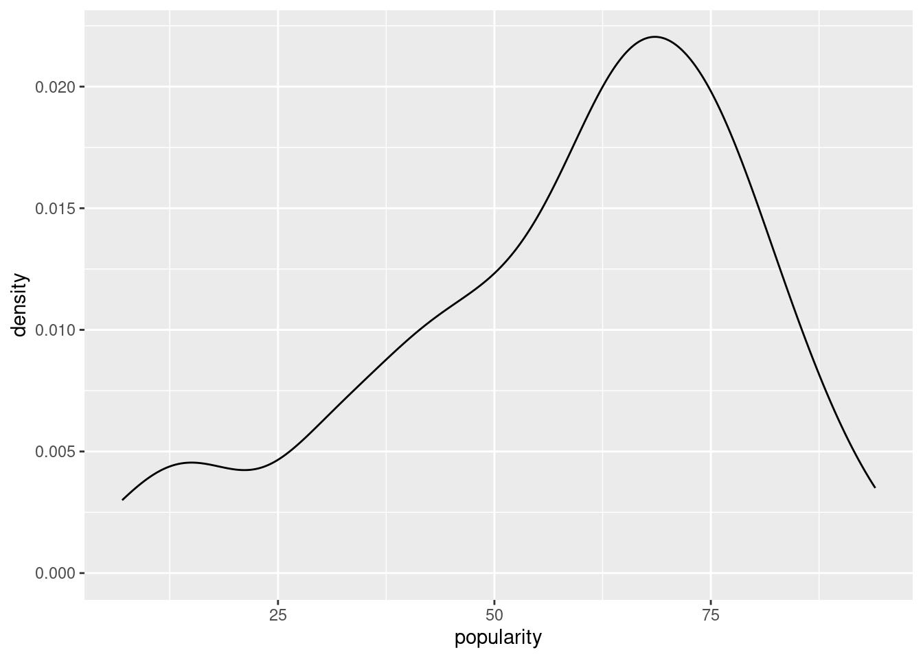
Even if the distribution is left skewed we will go with a Normal-Normal complete pooled model
\[Y_{ij}|\mu,\sigma \sim N (\mu, \sigma²)\]
\[\mu \sim N(50, 52^2)\]
\[\sigma \sim Exp(0.048)\]
\(\mu\) and \(\sigma\) are global parameter: they do not vary by artist:
\(\mu\): global mean popularity
\(\sigma\) : global standard deviation in popularity from song to song
spotify_complete_pooled <- stan_glm(
  popularity ~ 1,  # trick is here \mu = beta_0 (intercept) with no X
  data = spotify, family = gaussian,
  prior_intercept = normal(50, 2.5, # I do not understand 2.5
                           autoscale = TRUE),
  prior_aux = exponential(1, autoscale = TRUE),
  chains = 4, iter = 5000*2, seed = 84735)
complete_summary <- tidy(spotify_complete_pooled,
effects = c("fixed", "aux"),
conf.int = TRUE, conf.level = 0.80)
complete_summary## # A tibble: 3 × 5
## term estimate std.error conf.low conf.high
## <chr> <dbl> <dbl> <dbl> <dbl>
## 1 (Intercept) 58.4 1.10 57.0 59.8
## 2 sigma 20.7 0.776 19.7 21.7
## 3 mean_PPD 58.4 1.57 56.4 60.416.2.1 Quiz!!
3 artist:
- Mia X, artist with the lowest mean popularity in our data set
- Beyoncé, artist with nearly the highest mean popularity in our data set
- Mohsen Beats, an artist not in out data set
Using complete pooled model, what would be the approximate posterior predictive mean for a new song from this 3 artists?
artist_means <- spotify |>
group_by(artist) |>
summarize(count = n(), popularity = mean(popularity))
set.seed(84735)
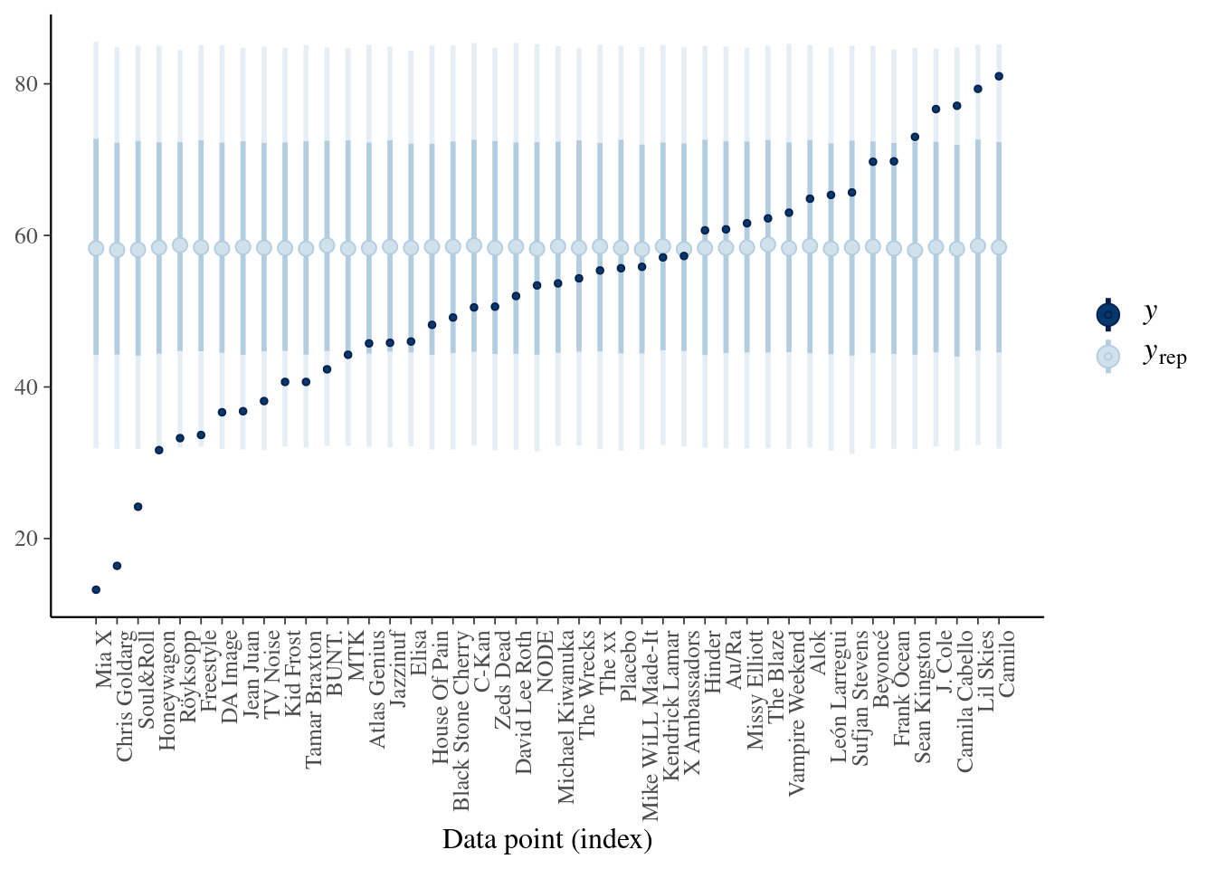
predictions_complete <- posterior_predict(spotify_complete_pooled,
newdata = artist_means)
ppc_intervals(artist_means$popularity, yrep = predictions_complete,
prob_outer = 0.80) +
ggplot2::scale_x_continuous(labels = artist_means$artist,
breaks = 1:nrow(artist_means)) +
xaxis_text(angle = 90, hjust = 1)