14.4 One Numerical Predictor

Let’s ignore the penguin’s weight for now and classify its species using only the fact that it has a 50mm-long bill

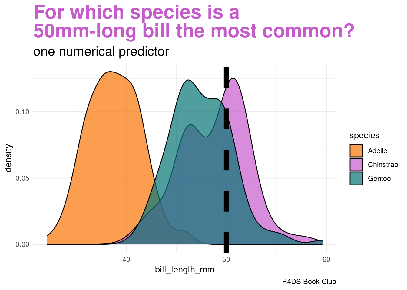
image code

penguins|>
  ggplot(aes(x = bill_length_mm, fill = species)) + 
  geom_density(alpha = 0.7) + 
  geom_vline(xintercept = 50, linetype = "dashed", linewidth = 3) + 
  labs(title = "<span style = 'color:#c65ccc'>For which species is a<br>50mm-long bill the most common?</span>",
       subtitle = "one numerical predictor",
       caption = "R4DS Book Club") +
  scale_fill_manual(values = c(adelie_color, chinstrap_color, gentoo_color)) +
  theme_minimal() +
  theme(plot.title = element_markdown(face = "bold", size = 24),
        plot.subtitle = element_markdown(size = 16))

Our data points to our penguin being a Chinstrap

we must weigh this data against the fact that Chinstraps are the rarest of these three species
difficult to compute likelihood \(L(y = A | x_{2} = 50)\)

This is where one “naive” part of naive Bayes classification comes into play. The naive Bayes method typically assumes that any quantitative predictor, here \(X_{2}\), is continuous and conditionally normal:

\[\begin{array}{rcl} X_{2} | (Y = A) & \sim & N(\mu_{A}, \sigma_{A}^{2}) \\ X_{2} | (Y = C) & \sim & N(\mu_{C}, \sigma_{C}^{2}) \\ X_{2} | (Y = G) & \sim & N(\mu_{G}, \sigma_{G}^{2}) \\ \end{array}\]

14.4.1 Prior Probability Distributions

# Calculate sample mean and sd for each Y group
penguins %>% 
  group_by(species) %>% 
  summarize(mean = mean(bill_length_mm, na.rm = TRUE), 
            sd = sd(bill_length_mm, na.rm = TRUE))

## # A tibble: 3 × 3
##   species    mean    sd
##   <fct>     <dbl> <dbl>
## 1 Adelie     38.8  2.66
## 2 Chinstrap  48.8  3.34
## 3 Gentoo     47.5  3.08

penguins |>
  ggplot(aes(x = bill_length_mm, color = species)) + 
  stat_function(fun = dnorm, args = list(mean = 38.8, sd = 2.66), 
                aes(color = "Adelie"), linewidth = 3) +
  stat_function(fun = dnorm, args = list(mean = 48.8, sd = 3.34),
                aes(color = "Chinstrap"), linewidth = 3) +
  stat_function(fun = dnorm, args = list(mean = 47.5, sd = 3.08),
                aes(color = "Gentoo"), linewidth = 3) +
  ...

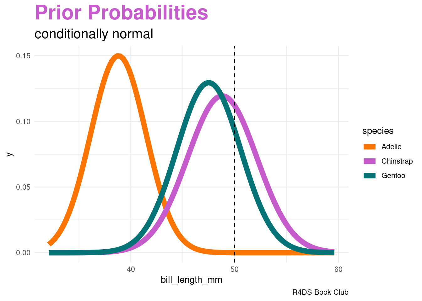
image code

penguins |>
  ggplot(aes(x = bill_length_mm, color = species)) + 
  stat_function(fun = dnorm, args = list(mean = 38.8, sd = 2.66), 
                aes(color = "Adelie"), linewidth = 3) +
  stat_function(fun = dnorm, args = list(mean = 48.8, sd = 3.34),
                aes(color = "Chinstrap"), linewidth = 3) +
  stat_function(fun = dnorm, args = list(mean = 47.5, sd = 3.08),
                aes(color = "Gentoo"), linewidth = 3) + 
  geom_vline(xintercept = 50, linetype = "dashed") + 
  labs(title = "<span style = 'color:#c65ccc'>Prior Probabilities</span>",
       subtitle = "conditionally normal",
       caption = "R4DS Book Club") +
  scale_color_manual(values = c(adelie_color, chinstrap_color, gentoo_color)) +
  theme_minimal() +
  theme(plot.title = element_markdown(face = "bold", size = 24),
        plot.subtitle = element_markdown(size = 16))

Computing the likelihoods in R:

# L(y = A | x_2 = 50) = 2.12e-05
dnorm(50, mean = 38.8, sd = 2.66)

# L(y = C | x_2 = 50) = 0.112
dnorm(50, mean = 48.8, sd = 3.34)

# L(y = G | x_2 = 50) = 0.09317
dnorm(50, mean = 47.5, sd = 3.08)

Total probability:

\[f(x_{2} = 50) = \frac{151}{342} \cdot 0.0000212 + \frac{68}{342} \cdot 0.112 + \frac{123}{342} \cdot 0.09317 \approx 0.05579\]

Bayes’ Rules:

\[\begin{array}{rcccccl} f(y = A | x_{2} = 50) & = & \frac{f(y = A) \cdot L(y = A | x_{1} = 0)}{f(x_{1} = 0)} = \frac{\frac{151}{342} \cdot 0.0000212}{0.05579} & \approx & 0.0002 \\ f(y = C | x_{2} = 50) & = & \frac{f(y = A) \cdot L(y = C | x_{1} = 0)}{f(x_{1} = 0)} = \frac{\frac{68}{342} \cdot 0.112}{0.05579} & \approx & 0.3992 \\ f(y = G | x_{2} = 50) & = & \frac{f(y = A) \cdot L(y = G | x_{1} = 0)}{f(x_{1} = 0)} = \frac{\frac{123}{342} \cdot 0.09317}{0.05579} & \approx & 0.6006 \\ \end{array}\]

Though a 50mm-long bill is relatively less common among Gentoo than among Chinstrap, it follows that our naive Bayes classification, based on our prior information and penguin’s bill length alone, is that this penguin is a Gentoo – it has the highest posterior probability.

We’ve now made two naive Bayes classifications of our penguin’s species, one based solely on the fact that our penguin has below-average weight and the other based solely on its 50mm-long bill (in addition to our prior information). And these classifications disagree: we classified the penguin as Adelie in the former analysis and Gentoo in the latter. This discrepancy indicates that there’s room for improvement in our naive Bayes classification method.