12.7 Interpretation

equality %>%
  add_fitted_draws(equality_model, n = 50) %>%
  ggplot(aes(x = percent_urban, y = laws, color = historical)) +
  geom_line(aes(y = .value, group = paste(historical, .draw)), 
              alpha = .1) +
  geom_point(data = equality) +
  labs(title = "Anti-Discrimination Laws",
       subtitle = "Human Rights Campaign State Equality Index",
       caption = "R4DS Bayes Rules book club") +
  scale_color_manual(values = c("blue", "red", "purple")) +
  theme_minimal()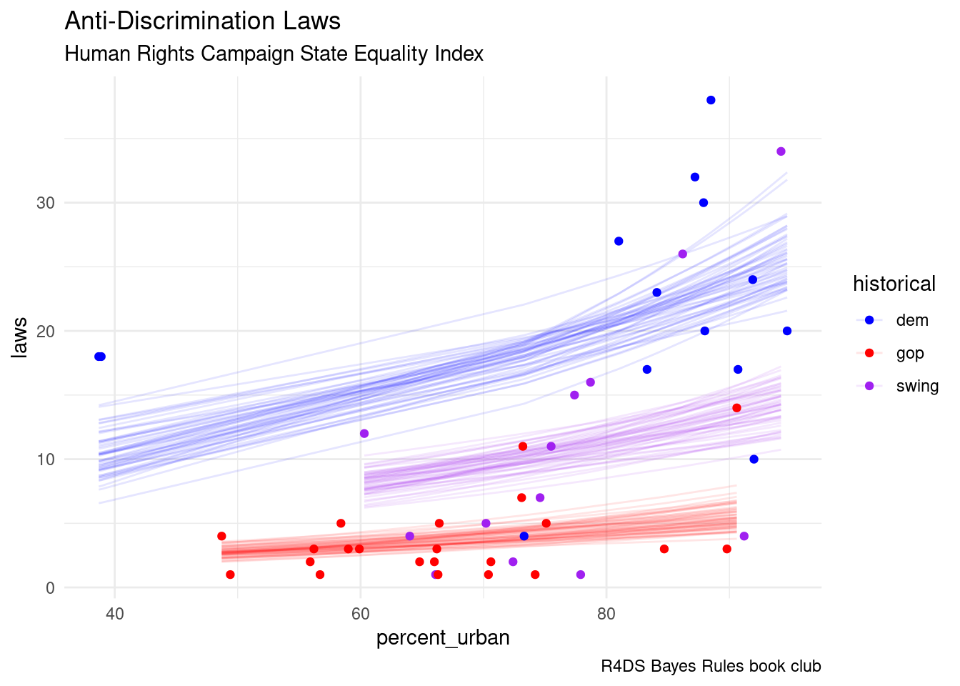

tidy(equality_model, conf.int = TRUE, conf.level = 0.80)

## # A tibble: 4 × 5
##   term            estimate std.error conf.low conf.high
##   <chr>              <dbl>     <dbl>    <dbl>     <dbl>
## 1 (Intercept)       1.71     0.303     1.31      2.09  
## 2 percent_urban     0.0164   0.00353   0.0119    0.0210
## 3 historicalgop    -1.52     0.134    -1.69     -1.34  
## 4 historicalswing  -0.610    0.103    -0.745    -0.477

\[\log(\lambda_{i}) = 1.71 + 0.0164X_{i1} - 1.52X_{i2} - 0.61X_{i3}\] or \[\lambda_{i} = e^{1.71 + 0.0161X_{i1} - 1.52X_{i2} - 0.61X_{i3}}\]

• \(\beta_{0} = 1.71\): the “typical state” has \(e^{1.71} \approx 5.53\) anti-discrimination laws
• \(\beta_{1} = 0.0164\): when controlling for historical voting trends, if the urban population in one state is 1 percentage point greater than another state, we’d expect it to have 1.0165 times the number of, or 1.65% more, anti-discrimination laws \[e^{0.0164} \approx 1.0165\]
• \(\beta_{2} = -1.52\): when controlling for historicalgop voting trends, if the urban population in one state is 1 percentage point greater than another state, we’d expect it to have about 88 percent fewer anti-discrimination laws \[e^{-1.52} \approx 0.2187\]
• \(\beta_{3} = 0.61\): when controlling for historicalswing voting trends, if the urban population in one state is 1 percentage point greater than another state, we’d expect it to have about 46 percent fewer anti-discrimination laws \[e^{-1.52} \approx 0.5434\]