13.13 The Family-Wise Error Rate

If the null hypothesis is true for each of \(m\) independent hypothesis tests, then the FWER is equal to \(1-(1-\alpha)^m\).

We can use this expression to compute the FWER for \(m=1,\ldots, 500\) and \(\alpha=0.05\), \(0.01\), and \(0.001\).

m <- 1:500
fwe1 <- 1 - (1 - 0.05)^m
fwe2 <- 1 - (1 - 0.01)^m
fwe3 <- 1 - (1 - 0.001)^m

We now conduct a one-sample \(t\)-test for each of the first five managers in the Fund dataset, in order to test the null hypothesis that the \(j\)th fund manager’s mean return equals zero, \(H_{0j}: \mu_j=0\).

library(ISLR2)
fund.mini <- Fund[, 1:5]

t.test(fund.mini[, 1], mu = 0)

## 
##  One Sample t-test
## 
## data:  fund.mini[, 1]
## t = 2.8604, df = 49, p-value = 0.006202
## alternative hypothesis: true mean is not equal to 0
## 95 percent confidence interval:
##  0.8923397 5.1076603
## sample estimates:
## mean of x 
##         3

fund.pvalue <- rep(0, 5)


for (i in 1:5)
  fund.pvalue[i] <- t.test(fund.mini[, i], mu = 0)$p.value

fund.pvalue

## [1] 0.006202355 0.918271152 0.011600983 0.600539601 0.755781508

We will make a correction with Bonferroni’s method and Holm’s method to control the FWER.

To do this, we use the p.adjust() function.

In other words, the adjusted \(p\)-values resulting from the p.adjust() function can be compared to the desired FWER in order to determine whether or not to reject each hypothesis.

p.adjust(fund.pvalue, method = "bonferroni")

## [1] 0.03101178 1.00000000 0.05800491 1.00000000 1.00000000

pmin(fund.pvalue * 5, 1)

## [1] 0.03101178 1.00000000 0.05800491 1.00000000 1.00000000

Therefore, using Bonferroni’s method, we are able to reject the null hypothesis only for Manager One while controlling the FWER at \(0.05\).

By contrast, using Holm’s method, the adjusted \(p\)-values indicate that we can reject the null hypotheses for Managers One and Three at a FWER of \(0.05\).

p.adjust(fund.pvalue, method = "holm")

## [1] 0.03101178 1.00000000 0.04640393 1.00000000 1.00000000

Manager One performs well, whereas Manager Two has poor performance.

apply(fund.mini, 2, mean)

## Manager1 Manager2 Manager3 Manager4 Manager5 
##      3.0     -0.1      2.8      0.5      0.3

t.test(fund.mini[, 1], fund.mini[, 2], paired = T)

## 
##  Paired t-test
## 
## data:  fund.mini[, 1] and fund.mini[, 2]
## t = 2.128, df = 49, p-value = 0.03839
## alternative hypothesis: true mean difference is not equal to 0
## 95 percent confidence interval:
##  0.1725378 6.0274622
## sample estimates:
## mean difference 
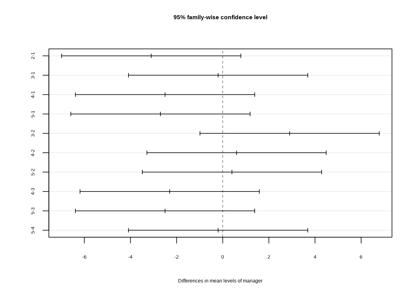
##             3.1

Here, we use the TukeyHSD() function to apply Tukey’s methodin order to adjust for multiple testing.

conflicted::conflict_prefer("as.matrix", "base")

## [conflicted] Will prefer base::as.matrix over any other package.

returns <- as.vector(base::as.matrix(fund.mini))
manager <- rep(c("1", "2", "3", "4", "5"), rep(50, 5))
a1 <- aov(returns ~ manager)
TukeyHSD(x = a1)

##   Tukey multiple comparisons of means
##     95% family-wise confidence level
## 
## Fit: aov(formula = returns ~ manager)
## 
## $manager
##     diff        lwr       upr     p adj
## 2-1 -3.1 -6.9865435 0.7865435 0.1861585
## 3-1 -0.2 -4.0865435 3.6865435 0.9999095
## 4-1 -2.5 -6.3865435 1.3865435 0.3948292
## 5-1 -2.7 -6.5865435 1.1865435 0.3151702
## 3-2  2.9 -0.9865435 6.7865435 0.2452611
## 4-2  0.6 -3.2865435 4.4865435 0.9932010
## 5-2  0.4 -3.4865435 4.2865435 0.9985924
## 4-3 -2.3 -6.1865435 1.5865435 0.4819994
## 5-3 -2.5 -6.3865435 1.3865435 0.3948292
## 5-4 -0.2 -4.0865435 3.6865435 0.9999095

mean(TukeyHSD(x = a1)$manager[,4])

## [1] 0.600986

The TukeyHSD() function provides confidence intervals for the difference between each pair of managers (lwr and upr), as well as a \(p\)-value.

All of these quantities have been adjusted for multiple testing.

Let’s plot the confidence intervals for the pairwise comparisons using the plot() function.

plot(TukeyHSD(x = a1))

---