13.15 A Re-Sampling Approach

Re-sampling approach to hypothesis testing using the Khan dataset.

attach(Khan)
x <- rbind(xtrain, xtest)
y <- c(as.numeric(ytrain), as.numeric(ytest))
dim(x)

## [1]   83 2308

table(y)

## y
##  1  2  3  4 
## 11 29 18 25

There are four classes of cancer.

For each gene, we compare the mean expression in the second class (rhabdomyosarcoma) to the mean expression in the fourth class (Burkitt’s lymphoma).

x <- as.matrix(x)
x1 <- x[which(y == 2), ]
x2 <- x[which(y == 4), ]
n1 <- nrow(x1)
n2 <- nrow(x2)
t.out <- t.test(x1[, 11], x2[, 11], var.equal = TRUE)
TT <- t.out$statistic
TT

##         t 
## -2.093633

t.out$p.value

## [1] 0.04118644

Instead of using this theoretical null distribution, we can randomly split the 54 patients into two groups of 29 and 25, and compute a new test statistic.

Repeating this process 10,000 times:

set.seed(1)
B <- 10000
Tbs <- rep(NA, B)
for (b in 1:B) {
   dat <- sample(c(x1[, 11], x2[, 11]))
   Tbs[b] <- t.test(dat[1:n1], dat[(n1 + 1):(n1 + n2)],
        var.equal = TRUE
      )$statistic
}
mean((abs(Tbs) >= abs(TT)))

## [1] 0.0416

This fraction, \(0.0416\), is our re-sampling-based \(p\)-value. It is almost identical to the \(p\)-value of \(0.0412\) obtained using the theoretical null distribution.

A histogram of the re-sampling-based test statistics:

hist(Tbs, breaks = 100, xlim = c(-4.2, 4.2), main = "",
    xlab = "Null Distribution of Test Statistic", col = 7)
lines(seq(-4.2, 4.2, len = 1000),
    dt(seq(-4.2, 4.2, len = 1000),
      df = (n1 + n2 - 2)
    ) * 1000, col = 2, lwd = 3)
abline(v = TT, col = 4, lwd = 2)
text(TT + 0.5, 350, paste("T = ", round(TT, 4), sep = ""),
    col = 4)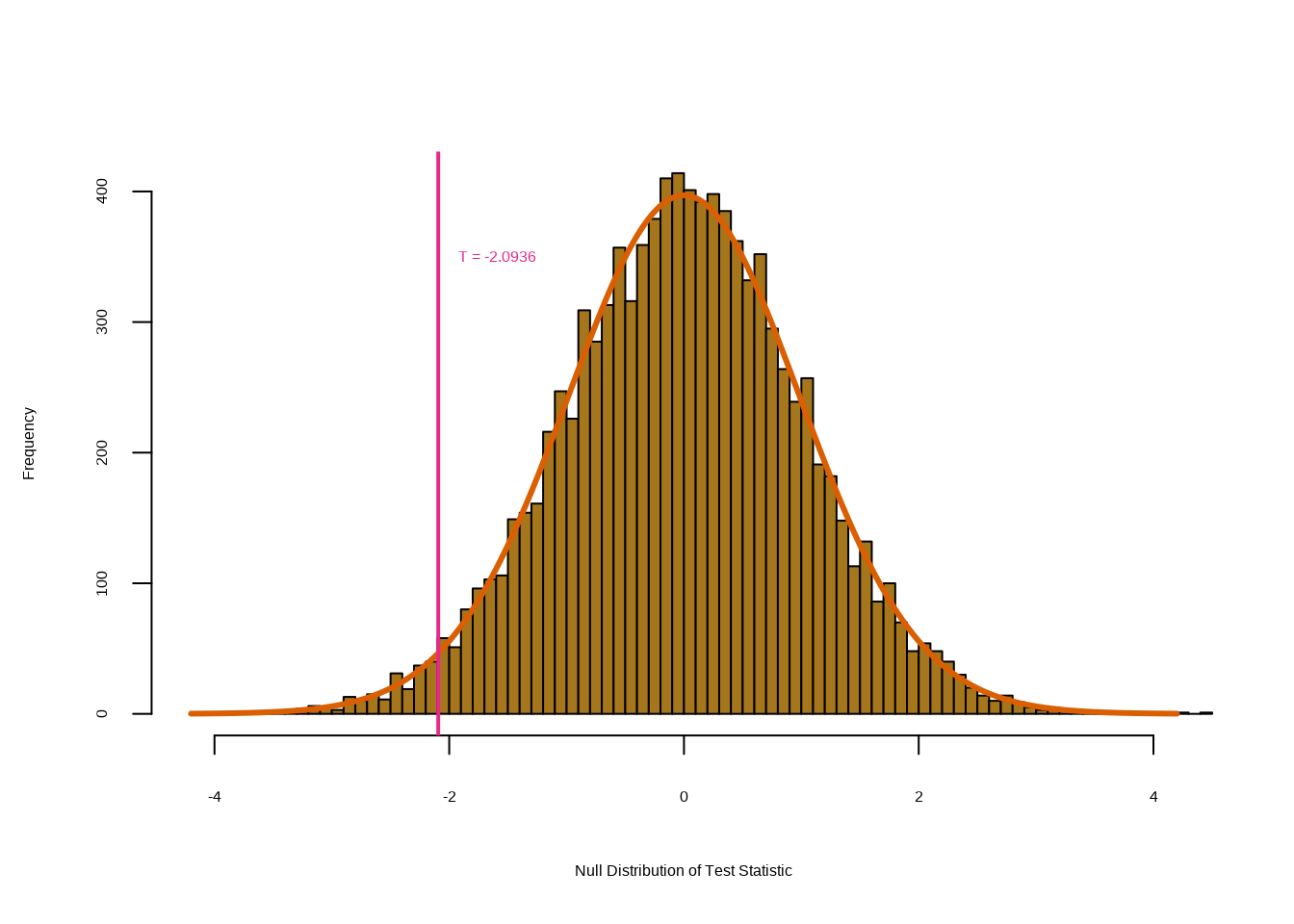

For each gene, we first compute the observed test statistic,

m <- 100
B<-1000
set.seed(1)
index <- sample(ncol(x1), m)
Ts <- rep(NA, m)
Ts.star <- matrix(NA, ncol = m, nrow = B)
for (j in 1:m) {
  k <- index[j]
  Ts[j] <- t.test(x1[, k], x2[, k],
        var.equal = TRUE
      )$statistic
  for (b in 1:B) {
    dat <- sample(c(x1[, k], x2[, k]))
    Ts.star[b, j] <- t.test(dat[1:n1],
         dat[(n1 + 1):(n1 + n2)], var.equal = TRUE
       )$statistic
  }
}

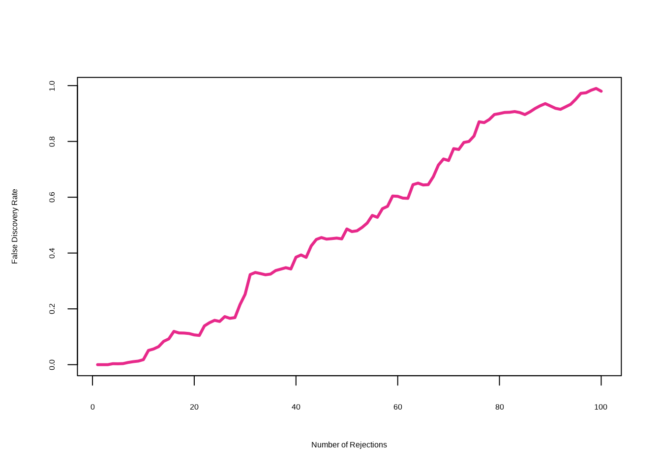
Compute a number of rejected null hypotheses \(R\).

cs <- sort(abs(Ts))
FDRs <- Rs <- Vs <- rep(NA, m)
for (j in 1:m) {
  R <- sum(abs(Ts) >= cs[j])
  V <- sum(abs(Ts.star) >= cs[j]) / B
  Rs[j] <- R
  Vs[j] <- V
  FDRs[j] <- V / R
}

The variable index is needed here since we restricted our analysis to just \(100\) randomly-selected genes.

max(Rs[FDRs <= .1])

## [1] 15

sort(index[abs(Ts) >= min(cs[FDRs < .1])])

##  [1]   29  465  501  554  573  729  733 1301 1317 1640 1646 1706 1799 1942 2159

max(Rs[FDRs <= .2])

## [1] 28

sort(index[abs(Ts) >= min(cs[FDRs < .2])])

##  [1]   29   40  287  361  369  465  501  554  573  679  729  733  990 1069 1073
## [16] 1301 1317 1414 1639 1640 1646 1706 1799 1826 1942 1974 2087 2159

plot(Rs, FDRs, xlab = "Number of Rejections", type = "l",
    ylab = "False Discovery Rate", col = 4, lwd = 3)

---