1.11 Datasets provided in the ISLR2 package
The book provides the {ISLR2} R package with all the datasets needed the analysis.
# install.packages("ISLR2")
# install.packages("remotes")
# remotes::install_github("r4ds/bookclub-islr")
# remove.packages("bookclubislr")
library(ISLR2)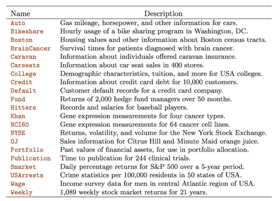
Figure 1.2: Datasets in ISLR2 package
1.11.1 Example datasets
As an example some of the data sets used are:
- Wage Data: predicting a continuous or quantitative output value (a regression problem) - Chapter3.
ISLR2::Wage %>% head()## year age maritl race education region
## 231655 2006 18 1. Never Married 1. White 1. < HS Grad 2. Middle Atlantic
## 86582 2004 24 1. Never Married 1. White 4. College Grad 2. Middle Atlantic
## 161300 2003 45 2. Married 1. White 3. Some College 2. Middle Atlantic
## 155159 2003 43 2. Married 3. Asian 4. College Grad 2. Middle Atlantic
## 11443 2005 50 4. Divorced 1. White 2. HS Grad 2. Middle Atlantic
## 376662 2008 54 2. Married 1. White 4. College Grad 2. Middle Atlantic
## jobclass health health_ins logwage wage
## 231655 1. Industrial 1. <=Good 2. No 4.318063 75.04315
## 86582 2. Information 2. >=Very Good 2. No 4.255273 70.47602
## 161300 1. Industrial 1. <=Good 1. Yes 4.875061 130.98218
## 155159 2. Information 2. >=Very Good 1. Yes 5.041393 154.68529
## 11443 2. Information 1. <=Good 1. Yes 4.318063 75.04315
## 376662 2. Information 2. >=Very Good 1. Yes 4.845098 127.11574p1 <- Wage %>%
ggplot(aes(x = age, y = wage)) +
geom_point(color = "grey55") +
geom_smooth() +
theme_bw()p2<-Wage %>%
ggplot(aes(x = year, y = wage)) +
geom_point(color = "grey55") +
geom_smooth(method = "lm") +
theme_bw()p3<-Wage %>%
ggplot(aes(x = education, y = wage)) +
geom_boxplot(aes(fill = education), show.legend = FALSE) +
theme_bw() +
theme(axis.text.x = element_text(size = 5))library(patchwork)
p1|p2|p3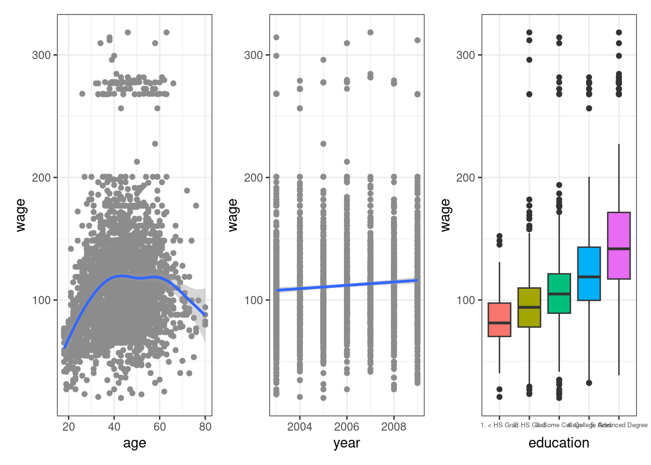
- Stock Market Data: predicting a categorical or qualitative output (classification problem). Predict whether the index will increase or decrease on a given day, using the past 5 days’ percentage changes in the index - Chapter 4.
ISLR2::Smarket %>% head()## Year Lag1 Lag2 Lag3 Lag4 Lag5 Volume Today Direction
## 1 2001 0.381 -0.192 -2.624 -1.055 5.010 1.1913 0.959 Up
## 2 2001 0.959 0.381 -0.192 -2.624 -1.055 1.2965 1.032 Up
## 3 2001 1.032 0.959 0.381 -0.192 -2.624 1.4112 -0.623 Down
## 4 2001 -0.623 1.032 0.959 0.381 -0.192 1.2760 0.614 Up
## 5 2001 0.614 -0.623 1.032 0.959 0.381 1.2057 0.213 Up
## 6 2001 0.213 0.614 -0.623 1.032 0.959 1.3491 1.392 UpSmarket %>%
pivot_longer(
cols=c("Lag1","Lag2","Lag3"), names_to="lags13", values_to="lags13_val"
) %>%
ggplot(aes(x=Direction,y=lags13_val)) +
geom_boxplot(aes(fill=Direction),show.legend = F) +
facet_wrap(~lags13) +
labs(x="Today's Direction",y="Percentage change in S&P") +
theme_bw() +
theme(strip.background = element_blank())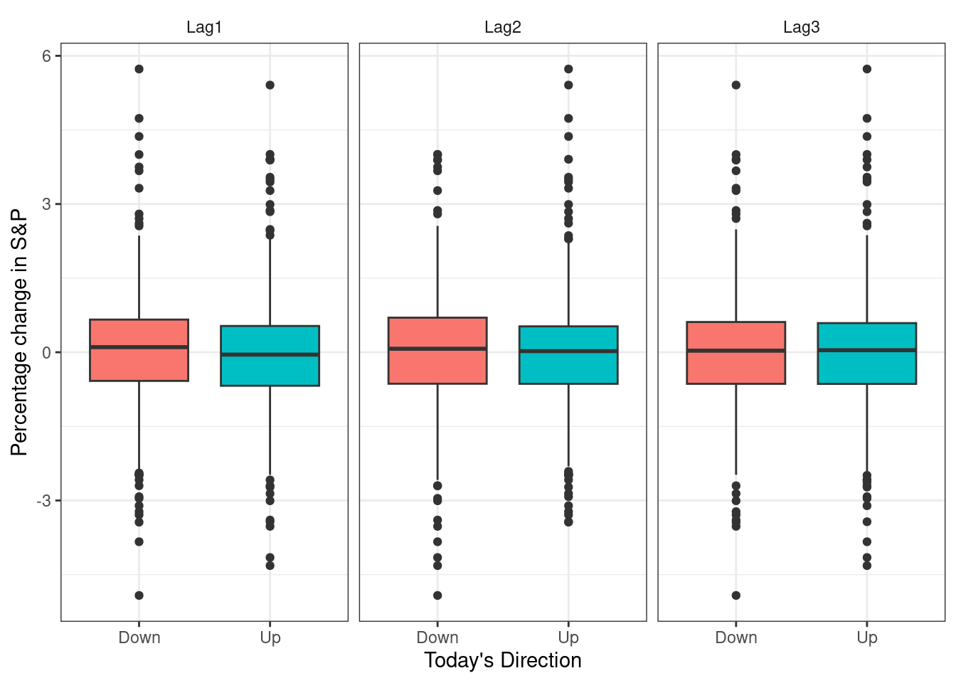
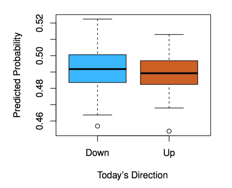
Figure 1.3: fit a quadratic discriminant analysis model
- Gene Expression Data
class(NCI60)## [1] "list"ISLR2::NCI60 %>% names()## [1] "data" "labs"NCI60$labs## [1] "CNS" "CNS" "CNS" "RENAL" "BREAST"
## [6] "CNS" "CNS" "BREAST" "NSCLC" "NSCLC"
## [11] "RENAL" "RENAL" "RENAL" "RENAL" "RENAL"
## [16] "RENAL" "RENAL" "BREAST" "NSCLC" "RENAL"
## [21] "UNKNOWN" "OVARIAN" "MELANOMA" "PROSTATE" "OVARIAN"
## [26] "OVARIAN" "OVARIAN" "OVARIAN" "OVARIAN" "PROSTATE"
## [31] "NSCLC" "NSCLC" "NSCLC" "LEUKEMIA" "K562B-repro"
## [36] "K562A-repro" "LEUKEMIA" "LEUKEMIA" "LEUKEMIA" "LEUKEMIA"
## [41] "LEUKEMIA" "COLON" "COLON" "COLON" "COLON"
## [46] "COLON" "COLON" "COLON" "MCF7A-repro" "BREAST"
## [51] "MCF7D-repro" "BREAST" "NSCLC" "NSCLC" "NSCLC"
## [56] "MELANOMA" "BREAST" "BREAST" "MELANOMA" "MELANOMA"
## [61] "MELANOMA" "MELANOMA" "MELANOMA" "MELANOMA"# View(NCI60)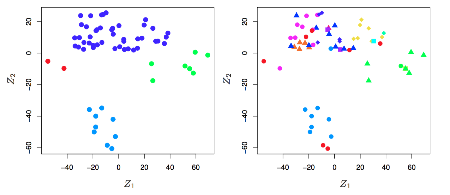
Figure 1.4: the first two principal components of the data