4.9 Linear regression with count data - heteroscedasticity

In this example, the variance of biker numbers changes as the mean number changes:

• during worse conditions, there are few bikers, and little variation in the number of bikers

• during better conditions, there are many bikers on average, but also larger variation in the number of bikers

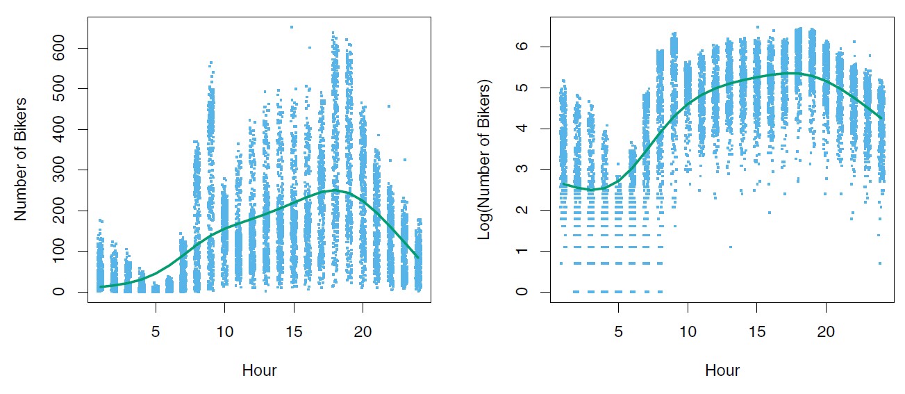
Figure 4.14: Left: On the Bikeshare dataset, the number of bikers is displayed on the y-axis, and the hour of the day is displayed on the x-axis. For the most part, as the mean number of bikers increases, so does the variance in the number of bikers. A smoothing spline fit is shown in green. Right: The log of the number of bikers is displayed on the y-axis.

Problem 2: observed heteroscedasticity is a violation of linear model assumptions

\[Y = \beta_{0} + \sum_{j=1}^p \beta_{j} + \epsilon\]

where \(\epsilon\) is a mean-zero error term with a constant variance

Transforming to log improves the variance, but cannot be used where the response can take on a 0 value.

Log transformation also results in challenges in interpretation:

e.g. “a one-unit increase in \(X_j\) is associated with an increase in the mean of the log of \(Y\) by an amount \(β_j\)”