7.4 Conceptual Exercises
- … cubic regression spline with a knot at \(x = \xi\) with basis functions
\[x, x^{2}, x^{3}, (x-\xi)_{+}^{3}\] where \[(x-\xi)_{+}^{3} = \begin{cases} (x-\xi)^{3} & x > \xi \\ 0 & \text{otherwise} \\ \end{cases}\]
We will show that a function of the form
\[f(x) = \beta_{0} + \beta_{1}x + \beta_{2}x^{2} + \beta_{3}x^{3} + \beta_{4}(x-\xi)_{+}^{3}\]
is indeed a cubic regression spline.
- Find a cubic polynomial
\[f_{1}(x) = a_{1} + b_{1}x + c_{1}x^{2} + d_{1}x^{3}\]
such that \(f_{1}(x) = f(x)\) for all \(x \leq \xi\).
Answer
\[\begin{array}{rcl} a_{1} & = & \beta_{0} \\ b_{1} & = & \beta_{1} \\ c_{1} & = & \beta_{2} \\ d_{1} & = & \beta_{3} \\ \end{array}\]
- Find a cubic polynomial
\[f_{2}(x) = a_{2} + b_{2}x + c_{2}x^{2} + d_{2}x^{3}\]
such that \(f_{2}(x) = f(x)\) for all \(x > \xi\).
Answer
\[\begin{array}{rcl} a_{2} & = & \beta_{0} - \beta_{4}\xi^{3} \\ b_{2} & = & \beta_{1} + 3\beta_{4}\xi^{2} \\ c_{2} & = & \beta_{2} - 3\beta_{4}\xi \\ d_{2} & = & \beta_{3} + \beta_{4} \\ \end{array}\]
We have now shown that \(f(x)\) is a piecewise polynomial.
- Show that \(f(x)\) is continuous at \(\xi\)
Answer
\[\begin{array}{rcl} f_{1}(\xi) & = & f_{2}(\xi) \\ \beta_{0} + \beta_{1}\xi + \beta_{2}\xi^{2} + \beta_{3}\xi^{3} & = & \beta_{0} + \beta_{1}\xi + \beta_{2}\xi^{2} + \beta_{3}\xi^{3} \\ \end{array}\]
- Show that \(f'(x)\) is continuous at \(\xi\)
Answer
\[\begin{array}{rcl} f_{1}'(\xi) & = & f_{2}'(\xi) \\ \beta_{1} + 2\beta_{2}\xi + 3\beta_{3}\xi^{2} & = & \beta_{1} + 2\beta_{2}\xi + 3\beta_{3}\xi^{2} \\ \end{array}\]
- Show that \(f''(x)\) is continuous at \(\xi\)
Answer
\[\begin{array}{rcl} f_{1}''(\xi) & = & f_{2}''(\xi) \\ 2\beta_{2} + 6\beta_{3}\xi & = & 2\beta_{2} + 6\beta_{3}\xi \\ \end{array}\]
- Suppose that a curve \(\hat{g}\) is computed to smoothly fit a set of \(n\) points using the following formula:
\[\hat{g} = \mathop{\mathrm{arg\,min}}_{g} \left( \displaystyle\sum_{i=1}^{n} (y_{i}-g(x_{i}))^{2} + \lambda\displaystyle\int \left[g^{(m)}(x)\right]^{2} \, dx \right)\]
where \(g^{(m)}\) is the \(m^{\text{th}}\) derivative of \(g\) (and \(g^{(0)} = g\)). Describe \(\hat{g}\) in each of the following situations.
- \(\lambda = \infty, \quad m = 0\)
Answer
heavy penalization of all functions except constants (i.e. horizontal lines)- \(\lambda = \infty, \quad m = 1\)
Answer
heavy penalization of all functions except linear functions—i.e. \[\hat{g} = a + bx\]- \(\lambda = \infty, \quad m = 2\)
Answer
heavy penalization of all functions except degree-2 polynomials \[\hat{g} = a + bx + cx^{2}\]- \(\lambda = \infty, \quad m = 3\)
Answer
heavy penalization of all functions except degree-3 polynomials \[\hat{g} = a + bx + cx^{2} + dx^{3}\]- \(\lambda = 0, \quad m = 2\)
Answer
No penalization implies perfect fit of training data.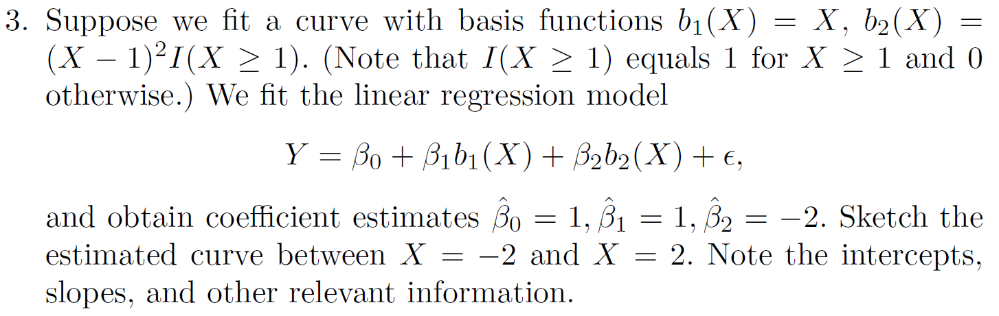
Answer
\[f(x) = \begin{cases} 1 + x, & -2 \leq x \leq 1 \\ 1 + x - 2(x-1)^{2}, & 1 \leq x \leq 2 \\ \end{cases}\]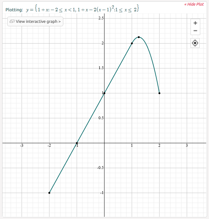
Answer
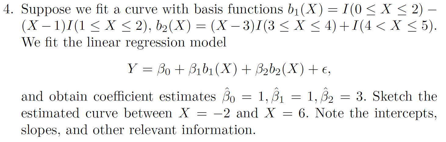
\[f(x) = \begin{cases} 0, & -2 \leq x < 0 \\ 1, & 0 \leq x \leq 1 \\ x, & 1 \leq x \leq 2 \\ 0, & 2 < x < 3 \\ 3x-3, & 3 \leq x \leq 4 \\ 1, & 4 < x \leq 5 \\ \end{cases}\]- Consider two curves \(\hat{g}_{1}\) and \(\hat{g}_{2}\)
\[\hat{g}_{1} = \mathop{\mathrm{arg\,min}}_{g} \left( \displaystyle\sum_{i=1}^{n} (y_{i}-g(x_{i}))^{2} + \lambda\displaystyle\int \left[g^{(3)}(x)\right]^{2} \, dx \right)\] \[\hat{g}_{2} = \mathop{\mathrm{arg\,min}}_{g} \left( \displaystyle\sum_{i=1}^{n} (y_{i}-g(x_{i}))^{2} + \lambda\displaystyle\int \left[g^{(4)}(x)\right]^{2} \, dx \right)\] where \(g^{(m)}\) is the \(m^{\text{th}}\) derivative of \(g\)
- As \(\lambda \rightarrow\infty\), will \(\hat{g}_{1}\) or \(\hat{g}_{2}\) have the smaller training RSS?
Answer
\(\hat{g}_{2}\) is more flexible due to the higher order of the penalty term than \(\hat{g}_{1}\), so \(\hat{g}_{2}\) will likely have a lower training RSS.- As \(\lambda \rightarrow\infty\), will \(\hat{g}_{1}\) or \(\hat{g}_{2}\) have the smaller testing RSS?
Answer
Generally, \(\hat{g}_{1}\) will perform better on less flexible functions, and \(\hat{g}_{2}\) will perform better on more flexible functions.- For \(\lambda = 0\), will \(\hat{g}_{1}\) or \(\hat{g}_{2}\) have the smaller training RSS?