3.4 Simple Linear Regression: Math

RSS = residual sum of squares

\[\mathrm{RSS} = e^{2}_{1} + e^{2}_{2} + \ldots + e^{2}_{n}\]

\[\mathrm{RSS} = (y_{1} - \hat{\beta}_{0} - \hat{\beta}_{1}x_{1})^{2} + (y_{2} - \hat{\beta}_{0} - \hat{\beta}_{1}x_{2})^{2} + \ldots + (y_{n} - \hat{\beta}_{0} - \hat{\beta}_{1}x_{n})^{2}\]

\[\hat{\beta}_{1} = \frac{\sum_{i=1}^{n}{(x_{i}-\bar{x})(y_{i}-\bar{y})}}{\sum_{i=1}^{n}{(x_{i}-\bar{x})^{2}}}\] \[\hat{\beta}_{0} = \bar{y} - \hat{\beta}_{1}\bar{x}\]

$\bar{x}$, $\bar{y}$ = sample means of $x$ and $y$

3.4.1 Visualization of Fit

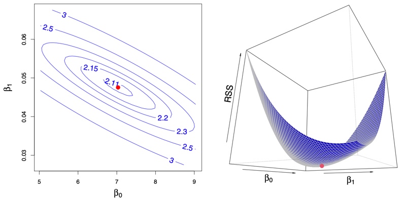
$Contour and three-dimensional plots of the RSS on the `Advertising` data, using `sales` as the response and `TV` as the predictor. The red dots correspond to the least squares estimates $\hat\beta_0$ and $\hat\beta_1$, given by (3.4)$

Figure 3.2: Contour and three-dimensional plots of the RSS on the Advertising data, using sales as the response and TV as the predictor. The red dots correspond to the least squares estimates $\hat\beta_0$ and $\hat\beta_1$, given by (3.4)

Learning Objectives:

Perform linear regression with a single predictor variable. ✔️