13.14 The False Discovery Rate

Now we perform hypothesis tests for all 2,000 fund managers in the Fund dataset.

With one-sample \(t\)-test of \(H_{0j}: \mu_j=0\), which states that the \(j\)th fund manager’s mean return is zero.

fund.pvalues <- rep(0, 2000)
for (i in 1:2000)
  fund.pvalues[i] <- t.test(Fund[, i], mu = 0)$p.value

The p.adjust() function can be used with Benjamini-Hochberg procedure.

q.values.BH <- p.adjust(fund.pvalues, method = "BH")
q.values.BH[1:10]

##  [1] 0.08988921 0.99149100 0.12211561 0.92342997 0.95603587 0.07513802
##  [7] 0.07670150 0.07513802 0.07513802 0.07513802

The q-values output by the Benjamini-Hochberg procedure can be interpreted as the smallest FDR threshold.

How many of the fund managers can we reject \(H_{0j}: \mu_j=0\)?

sum(q.values.BH <= .1)

## [1] 146

What if we had instead used Bonferroni’s method to control the FWER at level \(\alpha=0.1\)?

sum(fund.pvalues <= (0.1 / 2000))

## [1] 0

Finally, wh indexes all \(p\)-values that are less than or equal to the largest \(p\)-value in wh.ps. Therefore, whindexes the \(p\)-values rejected by the Benjamini-Hochberg procedure.

ps <- sort(fund.pvalues)
m <- length(fund.pvalues)
q <- 0.1
wh.ps <- which(ps < q * (1:m) / m)
if (length(wh.ps) >0) {
  wh <- 1:max(wh.ps)
 } else {
  wh <- numeric(0)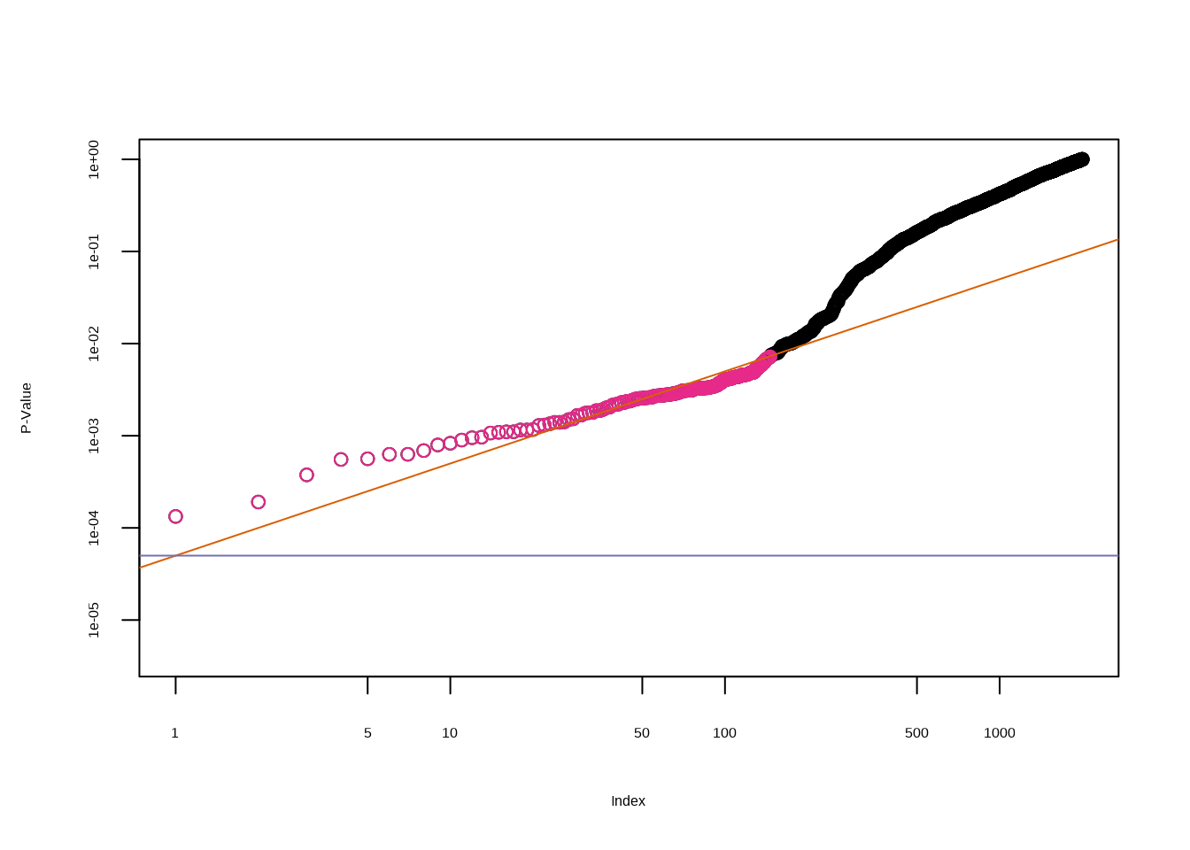
 }

plot(ps, log = "xy", ylim = c(4e-6, 1), ylab = "P-Value",
    xlab = "Index", main = "")
points(wh, ps[wh], col = 4)
abline(a = 0, b = (q / m), col = 2, untf = TRUE)
abline(h = 0.1 / 2000, col = 3)

---