13.10 Multiple T-test
For calculating the t-test for all the genes in the geneExpression matrix, we use the rowttests() function from the {genefilter} package.
?rowttestsWe define the NULL Hypothesis with a vector of the same length of the unique elements in the dataset. If our dataset is made of m unique elements and m0 are the number of positives, we can build a binary vector to use in the calculation of the pvalues.
Here is an example on how to make a nullHypothesis vector.
nullHypothesis <- c(rep(TRUE,m0), rep(FALSE,m-m0))
null_hypothesis <- factor(nullHypothesis, levels=c("TRUE","FALSE"))
In our case study we use the geneExpression matrix with genes expression data and the sampleInfo for retrieving the groups of positives and negatives within the dataset.
null_hypothesis <- factor(sampleInfo$group)Have a look a the dimentsion of the geneExpression matrix:
dim(geneExpression)## [1] 8793 24geneExpression%>%
as.data.frame() %>%
rownames_to_column("gene") %>%
count(gene,sort=T)%>%
head## gene n
## 1 1007_s_at 1
## 2 1053_at 1
## 3 117_at 1
## 4 121_at 1
## 5 1255_g_at 1
## 6 1294_at 1Statistics, difference in mean and p.value:
results <- rowttests(geneExpression,null_hypothesis)
results2 <- rowttests(geneExpression,factor(rep("a","b",24)))
results%>%head;results2%>%head
## statistic dm p.value
## 1007_s_at -2.11988375 -0.186257601 0.04553344
## 1053_at 2.26498355 0.226080913 0.03370683
## 117_at 1.54736766 0.096183548 0.13604026
## 121_at -0.54071279 -0.034530859 0.59413846
## 1255_g_at -0.03995292 -0.001775578 0.96849102
## 1294_at 1.80428848 0.154955035 0.08489586## statistic dm p.value
## 1007_s_at 136.6005 6.440704 5.687463e-35
## 1053_at 132.6100 7.187989 1.123837e-34
## 117_at 163.2384 5.224929 9.487983e-37
## 121_at 245.0113 7.702133 8.377450e-41
## 1255_g_at 148.2109 3.221102 8.729094e-36
## 1294_at 161.7306 7.277389 1.174338e-36The results is 1383 genes have a pvalue lower than 5%
results <- rowttests(geneExpression,null_hypothesis)
sum(results$p.value<0.05)mean(results$p.value<0.05)## [1] 0.157284213.10.1 FWER Family Wise Error Rate
What is the probability to make at least 1 type I error?
First consider the nuber of hypothesis which is the number of genes in our case:
m <- length(results$p.value)
m
## [1] 8793Then calculate the FWER:
1-(1-0.05)^m## [1] 1So, the probability to make at least one type I error is 1! if we set \(\alpha\): \[P(\text{at least one rejection})=1−(1−k)^m=5\%\] \[k=1-0.95^{\frac{1}{m}}\approx 0.000005\]
1-0.95^(1/m)## [1] 5.833407e-06What we need to do next is to adjust this FWER to a suitable threshold applying some corrections, such as the Bonferroni correction procedure sets \(k=\alpha/m\):
1-(1-0.05/m)^m## [1] 0.048770710.05/m## [1] 5.686341e-06sum(results$p.value<0.05/m)## [1] 10Now, the number of hypothesis with a pvalue lower than 5% are 10 and the FWER adjusted is:
mean(results$p.value<0.05/m)## [1] 0.00113726813.10.2 FDR False discovery rate
This is referred to as a discovery driven project or experiment, as we are now going to adjust the threshold to a lower value than \(\alpha\) through experiment just as the same as we have demonstrated above.
“The idea behind FDR is to focus on the random variable Q≡V/R with Q=0 when R=0 and V=0. Note that R=0 (nothing called significant) implies V=0 (no false positives). So Q is a random variable that can take values between 0 and 1 and we can define a rate by considering the average of Q. To better understand this concept here, we compute Q for the procedure: call everything p-value < 0.05 significant.”
Compare the FDR results for two methods.
- First method: using
p.adjust()function from {stats} package
pvals = results$p.value
pvals<-sort(pvals)

# to find a q-value with the false discovery rate method
fdr <- p.adjust(pvals, method="fdr")

sum(fdr<0.05)
## [1] 13mean(fdr<0.05)## [1] 0.001478449- Second method: using the
qvalue()function from {qvalue} package
res <- qvalue::qvalue(pvals)qvals <- res$qvalues
#plot(pvals,qvals)
sum(qvals<0.05)## [1] 22mean(qvals<0.05)## [1] 0.00250199The proportion of true null hypotheses:
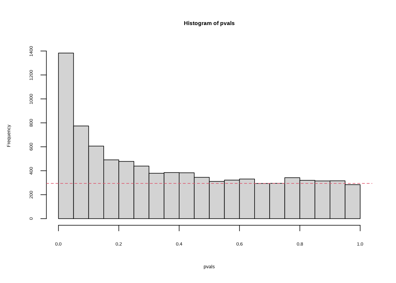
res$pi0## [1] 0.6695739hist(pvals,breaks=seq(0,1,len=21))
expectedfreq <- length(pvals)/20 #per bin
abline(h=expectedfreq*qvalue(pvals)$pi0,col=2,lty=2)