3.10 Potential Problems
Non-linear relationships
Residual plots are useful tool to see if any remaining trends exist. If so consider fitting transformation of the data.
Correlation of Error Terms
Linear regression assumes that the error terms \(\epsilon_i\) are uncorrelated. Residuals may indicate that this is not correct (obvious tracking in the data). One could also look at the autocorrelation of the residuals. What to do about it?
Non-constant variance of error terms
Again this can be revealed by examining the residuals. Consider transformation of the predictors to remove non-constant variance. The figure below shows residuals demonstrating non-constant variance, and shows this being mitigated to a great extent by log transforming the data.
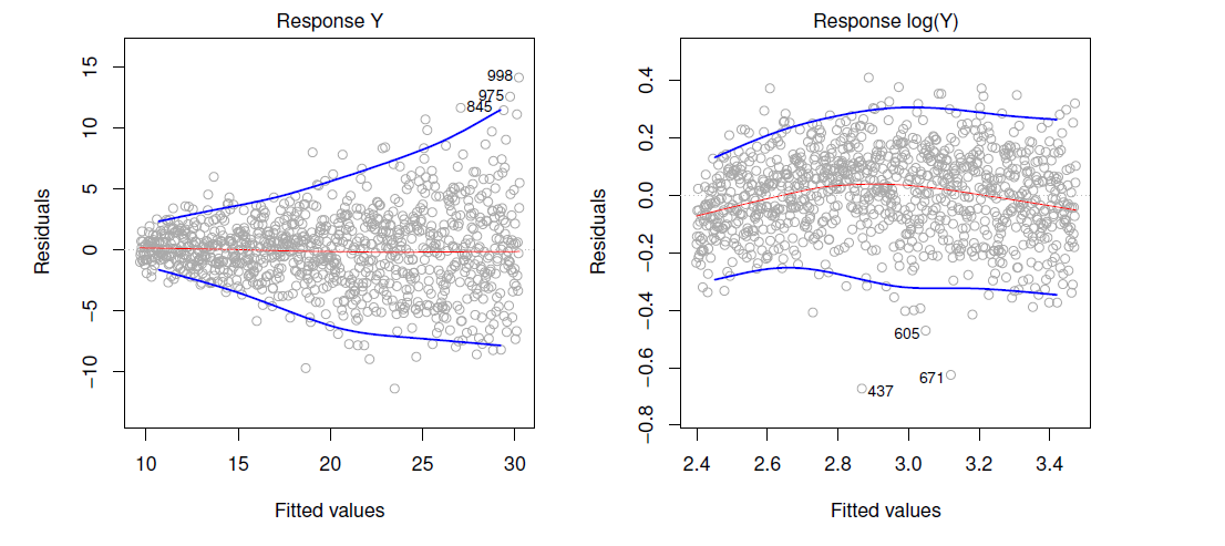
Figure 3.11 from book
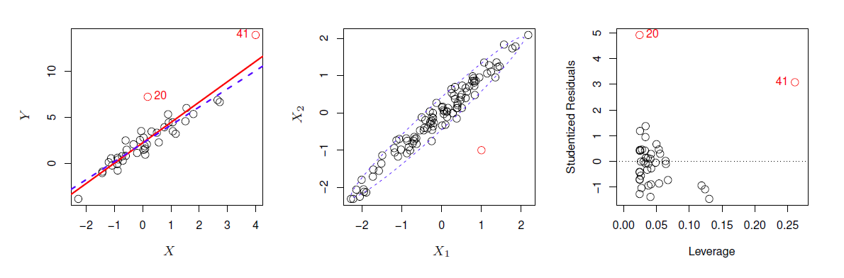
Outliers
- Outliers are points with for which \(y_i\) is far from value predicted by the model (including irreducible error). See point labeled ‘20’ in figure 3.13.
- Detect outliers by plotting studentized residuals (residual \(e_i\) divided by the estimated error) and look for residuals larger then 3 standard deviations in absolute value.
- An outlier may not effect the fit much but can have dramatic effect on the RSE.
- Often outliers are mistakes in data collection and can be removed, but could also be an indicator of a deficient model.
High Leverage Points
- These are points with unusual values of \(x_i\). Examples is point labeled ‘41’ in figure 3.13.
- These points can have large impact on the fit, as in the example, including point 41 pulls slope up significantly.
- Use leverage statistic to identify high leverage points, which can be hard to identify in multiple regression.
 6. Collinearity
- Two or more predictor variables are closely related to one another.
- Simple collinearity can be identified by looking at correlations between predictors.
- Causes the standard error to grow (and p-values to grow)
- Often can be dealt with by removing one of the highly correlated predictors or combining them.
- Multicollinearity (involving 3 or more predictors) is not so easy to identify. Use Variance inflation factor, which is the ratio of the variance of \(\hat{\beta_j}\) when fitting the full model to fitting the parameter on its own. Can be computed using the formula:
\[VIF(\hat{\beta_j}) = \frac{1}{1-R^2_{X_j|X_{-j}}}\] where \(R^2_{X_j|X_{-j}}\) is the \(R^2\) from a regression of \(X_j\) onto all the other predictors.