4.5 A Comparison of Classification Methods

Each of the classifiers below uses different estimates of $f_k(x)$.

linear discriminant analysis;
quadratic discriminant analysis;
naive Bayes

4.5.1 Linear Discriminant Analysis for p = 1

one predictor
classify an observation to the class for which $p_k(x)$ is greatest

Assumptions: - we assume that $f_k(x)$ is normal or Gaussian with a classs pecific mean and, - a shared variance term across all K classes [$σ^2_1 = · · · = σ^2_K$ ]

The normal density takes the form

\[f_k(x) = \frac{1}{\sqrt{2πσ_k}}exp(- \frac{1}{2σ^2_k}(x- \mu_k)^2)\]

Then, the posterior probability (probability that the observation belongs to the kth class, given the predictor value for that observation) is

\[p_k(x) = \frac{π_k \frac{1}{\sqrt{2πσ}}exp(- \frac{1}{2σ^2}(x- \mu_k)^2)}{\sum^k_{l=1} π_l \frac{1}{\sqrt{2πσ}}exp(- \frac{1}{2σ^2}(x- \mu_l)^2)}\]

Additional mathematical formula

After you log and rearrange the above equation, you will the following formula. The Bayes’ classifier assign to one class if $2x (μ_1 − μ_2) > μ_1^2 − μ_2^2$ and otherwise.

\[δ_k(x) = x . \frac{\mu_k}{\sigma^2} - \frac{\mu_k^2}{2\sigma^2} + log(π_k) \Longrightarrow {Equation \space 4.18}\]

The Bayes decision boundary is the point for which $δ_1(x) = δ_2(x)$

\[x = \frac{μ_1^2 − μ_2^2}{2(μ_1 − μ_2)} = \frac{μ_1 + μ_2}{2}\]

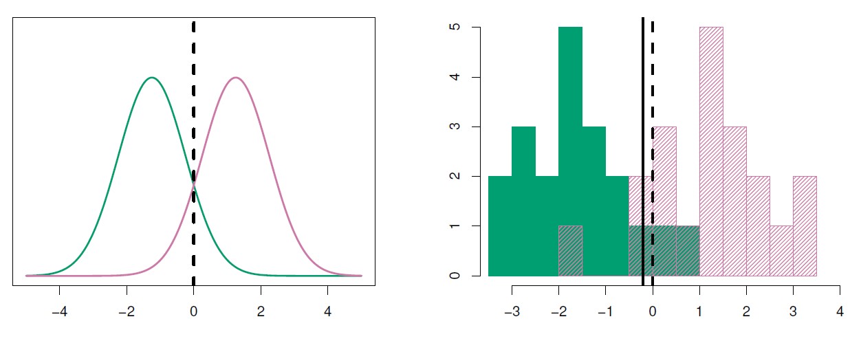
Left: Two one-dimensional normal density functions are shown. The dashed vertical line represents the Bayes decision boundary. Right: 20 observations were drawn from each of the two classes, and are shown as histograms. The Bayes decision boundary is again shown as a dashed vertical line. The solid vertical line represents the LDA decision boundary estimated from the training data.

Figure 4.4: Left: Two one-dimensional normal density functions are shown. The dashed vertical line represents the Bayes decision boundary. Right: 20 observations were drawn from each of the two classes, and are shown as histograms. The Bayes decision boundary is again shown as a dashed vertical line. The solid vertical line represents the LDA decision boundary estimated from the training data.

The linear discriminant analysis (LDA) method approximates the linear discriminant analysis Bayes classifier by plugging estimates for $π_k$, $μ_k$, and $σ^2$ into equation 4.18.

$\hat μ_k$ is the average of all the training observations from the kth class \[\hat{\mu}_{k} = \frac{1}{n_{k}}\sum_{i: y_{i}= k} x_{i}\]

$\hat σ^2$ is the weighted average of the sample variances for each of the K classes

\[\hat{\sigma}^2 = \frac{1}{n - K} \sum_{k = 1}^{K} \sum_{i: y_{i}= k} (x_{i} - \hat{\mu}_{k})^2\]

Note. n = total number of training observations, $n_k$ = number of training observations in the kth class

$π_k$ is estimated from the proportion of the training observations that belong to the kth class.

\[π_k = \frac{n_k}{n}\]

LDA classifier assigns an observation X = x to the class for which $δ_k(x)$ is largest.

\[δ_k(x) = x . \frac{\mu_k}{\sigma^2} - \frac{\mu_k^2}{2\sigma^2} + log(π_k) \Longrightarrow {Equation \space 4.18} \\ \Downarrow \\ \hat δ_k(x) = x \cdot \frac{\hat \mu_k}{\hat \sigma^2} - \frac{\hat \mu_k^2}{2\hat \sigma^2} + log(\hat π_k)\]

4.5.2 Linear Discriminant Analysis for p > 1

multiple predictors; p > 1 predictors
observations come from a multivariate Gaussian (or multivariate normal) distribution, with a class-specific mean vector and a common covariance matrix; \[N(μ_k,Σ)\]

Assumptions: - each individual predictor follows a one-dimensional normal distribution, with predictors having some correlation

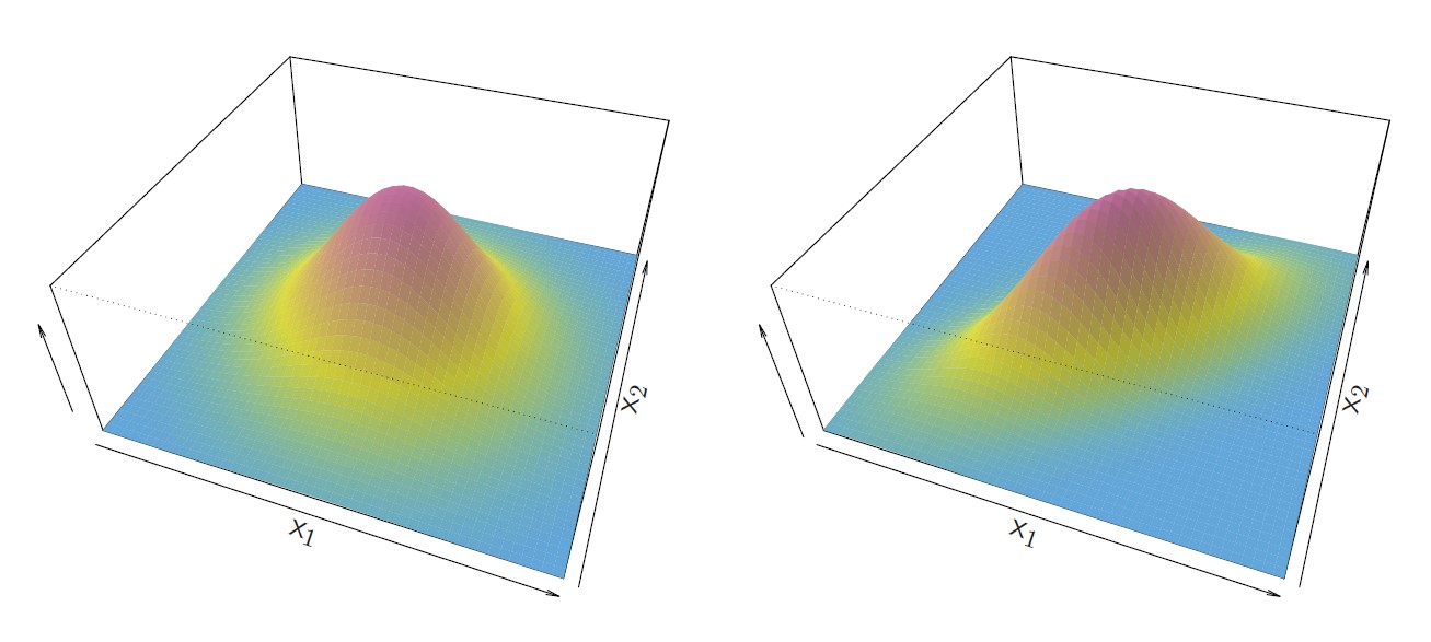
Two multivariate Gaussian density functions are shown, with p = 2. Left: The two predictors are uncorrelated and it has a circular base. Var(X_1) = Var(X_2) and Cor(X_1,X_2) = 0; Right: The two variables have a correlation of 0.7 with a elliptical base

Figure 4.5: Two multivariate Gaussian density functions are shown, with p = 2. Left: The two predictors are uncorrelated and it has a circular base. Var(X_1) = Var(X_2) and Cor(X_1,X_2) = 0; Right: The two variables have a correlation of 0.7 with a elliptical base

$\exp$ The multivariate Gaussian density is defined as:

\[f(x) = \frac{1}{(2π)^{\frac{p}{2}}|Σ|^{\frac{1}{2}}}\exp -\frac{1}{2}(x - \mu)^T Σ^{−1}(x − μ))\]

Bayes classifier assigns an observation X = x to the class for which \[δ_k(x)\] is largest.

\[δ_k(x) = x^T Σ^{−1}μ_k - \frac{1}{2}μ_k^T Σ^{−1} μ_k + log π_k \Longrightarrow vector/matrix \space version \\ δ_k(x) = x . \frac{\mu_k}{\sigma^2} - \frac{\mu_k^2}{2\sigma^2} + log(π_k) \Longrightarrow {Equation \space 4.18}\]

An example with three classes. The observations from each class are drawn from a multivariate Gaussian distribution with p = 2, with a class-specific mean vector and a common covariance matrix. Left: Ellipses that contain 95% of the probability for each of the three classes are shown. The dashed lines are the Bayes decision boundaries. Right: 20 observations were generated from each class, and the corresponding LDA decision boundaries are indicated using solid black lines. The Bayes decision boundaries are once again shown as dashed lines. Overall, the LDA decision boundaries are pretty close to the Bayes decision boundaries, shown again as dashed lines. The test error rates for the Bayes and LDA classifiers are 0.0746 and 0.0770, respectively.

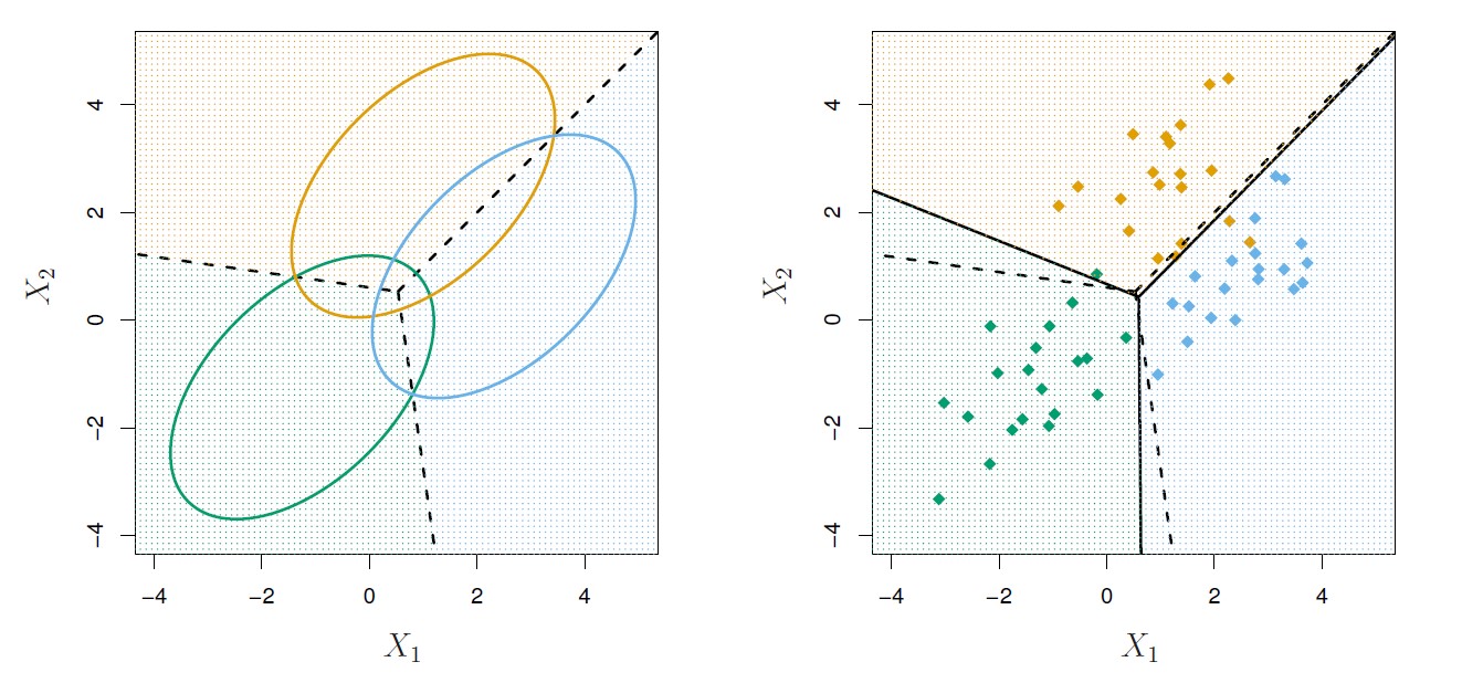
Figure 4.6: An example with three classes. The observations from each class are drawn from a multivariate Gaussian distribution with p = 2, with a class-specific mean vector and a common covariance matrix. Left: Ellipses that contain 95% of the probability for each of the three classes are shown. The dashed lines are the Bayes decision boundaries. Right: 20 observations were generated from each class, and the corresponding LDA decision boundaries are indicated using solid black lines. The Bayes decision boundaries are once again shown as dashed lines. Overall, the LDA decision boundaries are pretty close to the Bayes decision boundaries, shown again as dashed lines. The test error rates for the Bayes and LDA classifiers are 0.0746 and 0.0770, respectively.

All classification models have training error rate, which can be displayed with a confusion matrix.

Caveats of error rate:

training error rates will usually be lower than test error rates, which are the real quantity of interest. The higher the ratio of parameters p to number of samples n, the more we expect this overfitting to play a role.
the trivial null classifier will achieve an error rate that is only a bit higher than the LDA training set error rate
a binary classifier such as this one can make two types of errors (Type I and II)
Class-specific performance (sensitivity and specificity) is important in certain fields (e.g., medicine)

LDA has low sensitivity due to 1. LDA is trying to approximate the Bayes classifier, which has the lowest total error rate out of all classifiers 2. In the process, the Bayes classifier will yield the smallest possible total number of misclassified observations, regardless of the class from which the errors stem. 3. It also uses a threshold of 50% for the posterior probability of default in order to assign an observation to the default class

\[Pr(default = Yes|X = x) > 0.5. \\ Pr(default = Yes|X = x) > 0.2.\]

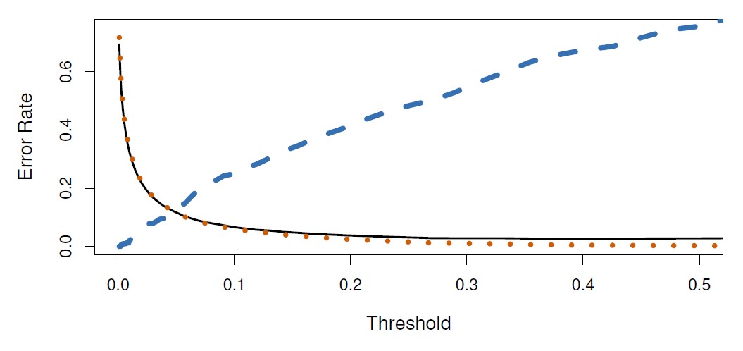
$The figure illustrates the trade-off that results from modifying the threshold value for the posterior probability of default. For the Default data set, error rates are shown as a function of the threshold value for the posterior probability that is used to perform the assignment. The black solid line displays the overall error rate. The blue dashed line represents the fraction of defaulting customers that are incorrectly classified, and the orange dotted line indicates the fraction of errors among the non-defaulting customers.$

Figure 4.7: The figure illustrates the trade-off that results from modifying the threshold value for the posterior probability of default. For the Default data set, error rates are shown as a function of the threshold value for the posterior probability that is used to perform the assignment. The black solid line displays the overall error rate. The blue dashed line represents the fraction of defaulting customers that are incorrectly classified, and the orange dotted line indicates the fraction of errors among the non-defaulting customers.

As the threshold is reduced, the error rate among individuals who default decreases steadily, but the error rate among the individuals who do not default increases. The decision on the threshold must be based on domain knowledge (e.g., detailed information about the costs associated with default)
ROC curve is a way to illustrate the two type of errors at all possible thresholds.

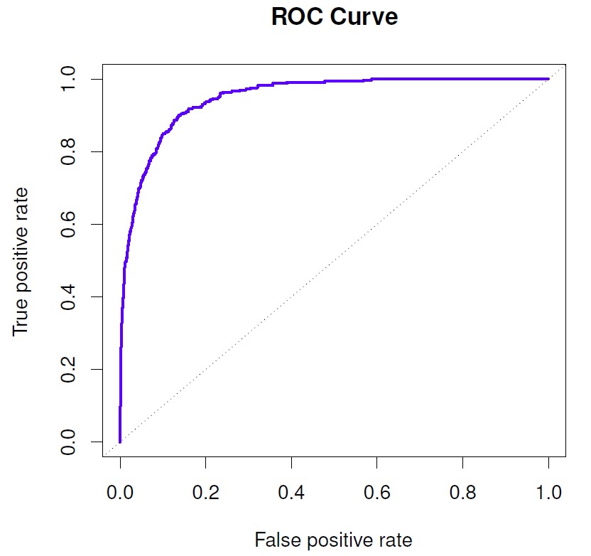
$The true positive rate is the sensitivity: the fraction of defaulters that are correctly identified, using a given threshold value. The false positive rate is 1-specificity: the fraction of non-defaulters that we classify incorrectly as defaulters, using that same threshold value. The ideal ROC curve hugs the top left corner, indicating a high true positive rate and a low false positive rate. The dotted line represents the “no information” classifier; this is what we would expect if student status and credit card balance are not associated with probability of default.$

Figure 4.8: The true positive rate is the sensitivity: the fraction of defaulters that are correctly identified, using a given threshold value. The false positive rate is 1-specificity: the fraction of non-defaulters that we classify incorrectly as defaulters, using that same threshold value. The ideal ROC curve hugs the top left corner, indicating a high true positive rate and a low false positive rate. The dotted line represents the “no information” classifier; this is what we would expect if student status and credit card balance are not associated with probability of default.

An ideal ROC curve will hug the top left corner, so the larger area under the ROC curve (AUC), the better the classifier.

	True class
	Neg. or Null	Pos. or Non-null	Total
Predicted class
− or Null	True Neg. (TN)	False Neg. (FN)	N∗
+ or Non-null	False Pos. (FP)	True Pos. (TP)	P∗
Total	N	P

Important measures for classification and diagnostic testing:

False Positive rate (FP/N) $\Longrightarrow$ Type I error, 1−Specificity
True Positive rate (TP/P) $\Longrightarrow$ 1−Type II error, power, sensitivity, recall
Pos. Predicted value (TP/P∗) $\Longrightarrow$ Precision, 1−false discovery proportion
Neg. Predicted value (TN/N∗)

4.5.3 Quadratic Discriminant Analysis (QDA)

Assumptions similar to LDA, in which observations from each class are drawn from a Gaussian distribution, and plugging estimates for the parameters into Bayes’ theorem in order to perform prediction
QDA assumes that each class has its own covariance matrix

\[X ∼ N(μ_k,Σ_k) \Longrightarrow {Σ_k is \space covariance \space matrix \space for \space the \space kth \space class}\]

Bayes classifier

\[δ_k(x) = - \frac{1}{2}(x - \mu_k)^T Σ_k^{−1}(x - \mu_k) - \frac{1}{2}log|Σ_k| + log(π_k) \\ \Downarrow \\ δ_k(x) = - \frac{1}{2}x^T Σ_k^{−1}x - x^T Σ_k^{−1} \mu_k - \frac{1}{2}μ_k^T Σ_k^{−1} μ_k - \frac{1}{2}log|Σ_k| + log π_k\]

QDA classifier involves plugging estimates for $Σ_k$, $μ_k$, and $π_k$ into the above equation, and then assigning an observation X = x to the class for which this quantity is largest.

The quantity x appears as a quadratic function, hence the name.

Why the LDA to QDA is preferred or vice-versa?
1. Bias-variance trade-off
- Pro LDA: LDA assumes that the K classes share a common covariance matrix and the quantity X becomes linear, which means there are $K_p$ linear coefficients to estimate.LDA is a much less flexible classifier than QDA, and so has substantially lower variance; improved prediction performance.

Con LDA: If the assumption K classes share a common covariance matrix is badly off, LDA can suffer from high bias
Conclusion: Use LDA when there is a few training observations; use QDA when the training set is very large or common covariance matrix is untennable.

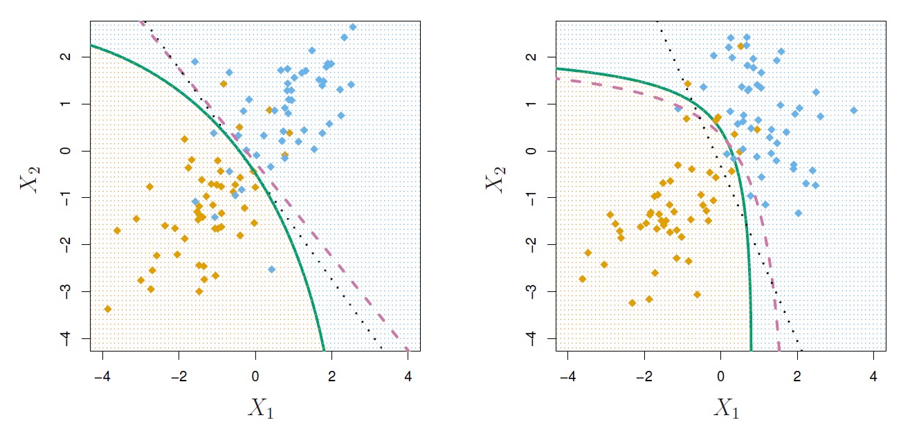
Left: The Bayes (purple dashed), LDA (black dotted), and QDA (green solid) decision boundaries for a two-class problem with Σ1 = Σ2. The shading indicates the QDA decision rule. Since the Bayes decision boundary is linear, it is more accurately approximated by LDA than by QDA. Right: Details are as given in the left-hand panel, except that Σ1 ̸= Σ2. Since the Bayes decision boundary is non-linear, it is more accurately approximated by QDA than by LDA.

Figure 4.9: Left: The Bayes (purple dashed), LDA (black dotted), and QDA (green solid) decision boundaries for a two-class problem with Σ1 = Σ2. The shading indicates the QDA decision rule. Since the Bayes decision boundary is linear, it is more accurately approximated by LDA than by QDA. Right: Details are as given in the left-hand panel, except that Σ1 ̸= Σ2. Since the Bayes decision boundary is non-linear, it is more accurately approximated by QDA than by LDA.

4.5.4 Naive Bayes

Estimating a p-dimensional density function is challenging; naive bayes make a different assumption than LDA and QDA.
an alternative to LDA that does not assume normally distributed predictors

\[f_k(x) = f_{k1}(x_1) × f_{k2}(x_2)×· · ·×f{k_p}(x_p),\] where $f_{kj}$ is the density function of the jth predictor among observations in the kth class

Within the kth class, the p predictors are independent.

Why naive Bayes is better/powerful?

By assuming that the p covariates are independent within each class, we assumed that there is no association between the predictors! When estimating a p-dimensional density function, it is difficult to calculate the marginal distribution of each predictor and joint distribution of the predictors.
Although p covariates might not be independent within each class, it is convenient and we obtain pretty decent results when the n is small, p is large.
It reduces variance, though it has some bias (Bias-variance trade-off)

Options to estimate the one-dimensional density function fkj using training data

[For Quantitative $X_j$] -> We assume $X_j |Y = k ∼ N(μ_{jk},σ_{jk}^2)$, where within each class, the jth predictor is drawn from a (univariate) normal distribution. It is QDA-like with diagonal class-specific covariance matrix
[For Quantitative $X_j$] -> Use a non-parametric estimate for $f_{kj}$. First, a histogram for the within-class observations and then estimate $f_{kj}(x_j)$. Or else, use kernel density estimator.
[For Qualitative $X_j$] ->Count the proportion of training observations for the jth predictor corresponding to each class.

Note: Fixing the threshold, the Naive Bayes has a higher error rate than LDA, but better prediction (higher sensitivity).