7.3 Generalized Additive Models
Generalized additive models were originally invented by Trevor Hastie and Robert Tibshirani in 1986 as a natural way to extend the conventional multiple linear regression model
\[ y_i = \beta_0+\beta_1x_{i1}+\beta_2x_{i2}...+\beta_px_{ip}+\epsilon_i\]
Mathematically speaking, GAM is an additive modeling technique where the impact of the predictive variables is captured through smooth functions which, depending on the underlying patterns in the data, can be nonlinear:

We can write the GAM structure as:
\[g(E(Y))=\alpha + s_1(x_1)+...+s_p(x_p) \]
where \(Y\) is the dependent variable (i.e., what we are trying to predict), \(E(Y)\) denotes the expected value, and \(g(Y)\) denotes the link function that links the expected value to the predictor variables \(x_1,…,x_p\).
The terms \(s_1(x_1),…,s_p(x_p)\) denote smooth, nonparametric functions. Note that, in the context of regression models, the terminology nonparametric means that the shape of predictor functions are fully determined by the data as opposed to parametric functions that are defined by a typically small set of parameters. This can allow for more flexible estimation of the underlying predictive patterns without knowing upfront what these patterns look like.
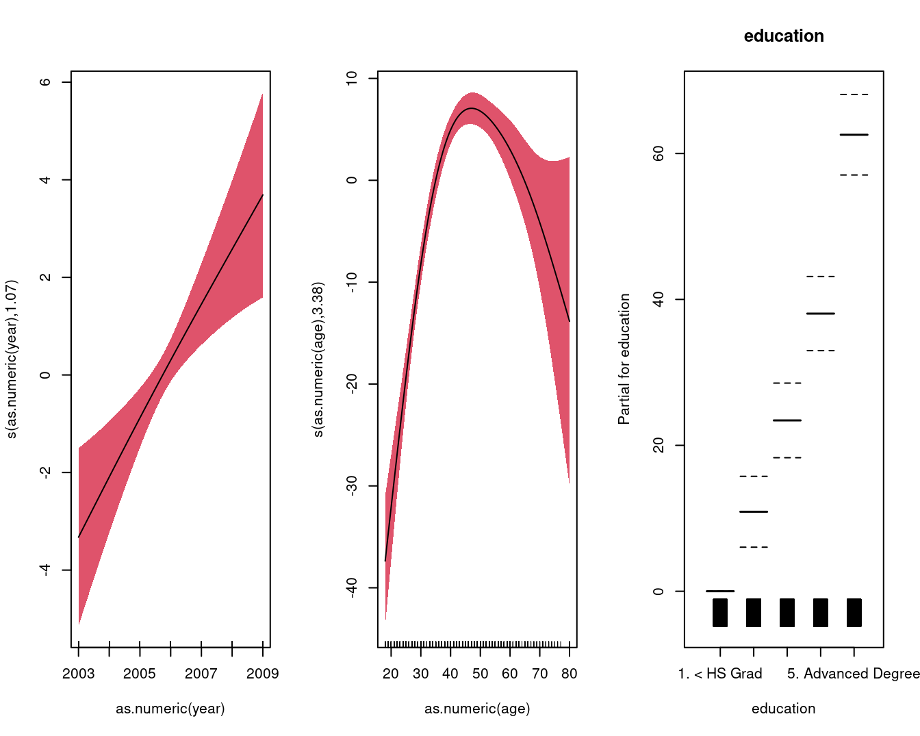
The mgcv version:
gam.m3 <-
  mgcv::gam(wage ~ s(as.numeric(year), k = 4) + s(as.numeric(age), k = 5) + education, data = Wage)

summary(gam.m3)
##
## Family: gaussian
## Link function: identity
##
## Formula:
## wage ~ s(as.numeric(year), k = 4) + s(as.numeric(age), k = 5) +
## education
##
## Parametric coefficients:
## Estimate Std. Error t value Pr(>|t|)
## (Intercept) 85.529 2.152 39.746 < 2e-16 ***
## education2. HS Grad 10.896 2.429 4.487 7.51e-06 ***
## education3. Some College 23.415 2.556 9.159 < 2e-16 ***
## education4. College Grad 38.058 2.541 14.980 < 2e-16 ***
## education5. Advanced Degree 62.568 2.759 22.682 < 2e-16 ***
## ---
## Signif. codes: 0 '***' 0.001 '**' 0.01 '*' 0.05 '.' 0.1 ' ' 1
##
## Approximate significance of smooth terms:
## edf Ref.df F p-value
## s(as.numeric(year)) 1.073 1.142 11.44 0.000392 ***
## s(as.numeric(age)) 3.381 3.787 57.96 < 2e-16 ***
## ---
## Signif. codes: 0 '***' 0.001 '**' 0.01 '*' 0.05 '.' 0.1 ' ' 1
##
## R-sq.(adj) = 0.289 Deviance explained = 29.1%
## GCV = 1241.3 Scale est. = 1237.4 n = 3000par(mfrow = c(1, 3))
mgcv::plot.gam(
gam.m3,
residuals = FALSE,
all.terms = TRUE,
shade = TRUE,
shade.col = 2,
rug = TRUE,
scale = 0
)
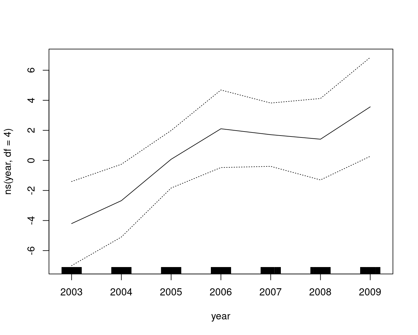
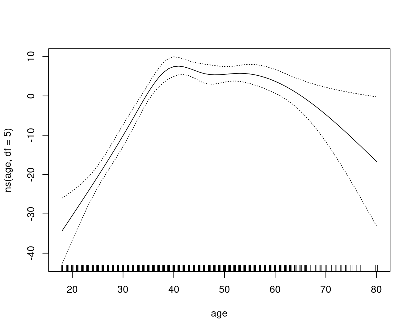
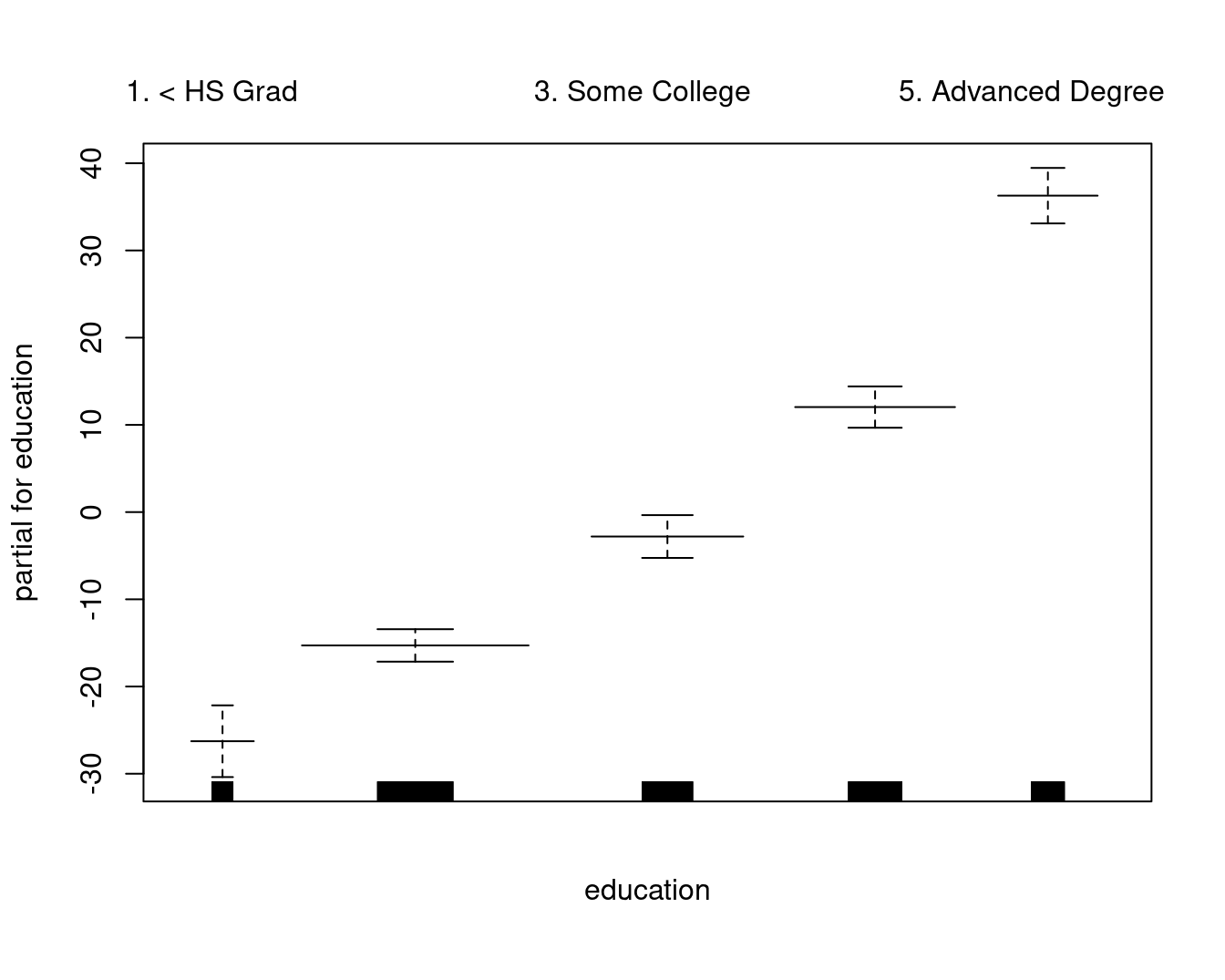
A comparable model, built with lm and natural cubic splines, plotted as the GAM contributions to the wage:
gam::plot.Gam(
  lm(wage ~ ns(year, df = 4) + ns(age, df = 5) + education, data = Wage),
  residuals = FALSE,
  rugplot = TRUE,
  se = TRUE,
  scale = 0
)
Why Use GAMs?
There are at least three good reasons why you want to use GAM: interpretability, flexibility/automation, and regularization. Hence, when your model contains nonlinear effects, GAM provides a regularized and interpretable solution, while other methods generally lack at least one of these three features. In other words, GAMs strike a nice balance between the interpretable, yet biased, linear model, and the extremely flexible, “black box” learning algorithms.
Coefficients not that interesting; fitted functions are.
Can mix terms — some linear, some nonlinear
Can use smoothing splines AND local regression as well
GAMs are simply additive, although low-order interactions can be included in a natural way using, e.g. bivariate smoothers or interactions
Fitting GAMs in R
The two main packages in R that can be used to fit generalized additive models are gam and mgcv. The gam package was written by Trevor Hastie and is more or less frequentist. The mgcv package was written by Simon Wood, and, while it follows the same framework in many ways, it is much more general because it considers GAM to be any penalized GLM (and Bayesian). The differences are described in detail in the documentation for mgcv.
I discovered that gam and mgcv do not work well when loaded at the same time. Restart the R session if you want to switch between the two packages – detaching one of the packages is not sufficient.
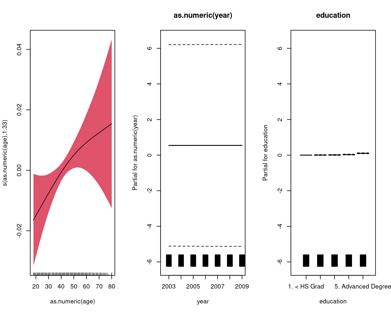
An example of a classification GAM model:
gam.lr <-
  mgcv::gam(I(wage > 250) ~ as.numeric(year) + s(as.numeric(age), k = 5) + education, data = Wage)

summary(gam.lr)
##
## Family: gaussian
## Link function: identity
##
## Formula:
## I(wage > 250) ~ as.numeric(year) + s(as.numeric(age), k = 5) +
## education
##
## Parametric coefficients:
## Estimate Std. Error t value Pr(>|t|)
## (Intercept) -0.5459574 2.8324135 -0.193 0.84717
## as.numeric(year) 0.0002724 0.0014121 0.193 0.84702
## education2. HS Grad 0.0048026 0.0107994 0.445 0.65656
## education3. Some College 0.0111980 0.0113639 0.985 0.32451
## education4. College Grad 0.0313156 0.0112829 2.775 0.00555 **
## education5. Advanced Degree 0.1034530 0.0122366 8.454 < 2e-16 ***
## ---
## Signif. codes: 0 '***' 0.001 '**' 0.01 '*' 0.05 '.' 0.1 ' ' 1
##
## Approximate significance of smooth terms:
## edf Ref.df F p-value
## s(as.numeric(age)) 1.333 1.593 2.896 0.0439 *
## ---
## Signif. codes: 0 '***' 0.001 '**' 0.01 '*' 0.05 '.' 0.1 ' ' 1
##
## R-sq.(adj) = 0.0452 Deviance explained = 4.73%
## GCV = 0.024548 Scale est. = 0.024488 n = 3000par(mfrow = c(1, 3))
mgcv::plot.gam(
gam.lr,
residuals = FALSE,
all.terms = TRUE,
shade = TRUE,
shade.col = 2,
rug = TRUE,
scale = 0
)